Automated Finite Element Analyses for Structural Integrated Systems

Chongyul Yoon

doi:10.7734/COSEIK.2024.37.1.49

Preview

Research Paper

Journal of the Computational Structural Engineering Institute of Korea. 29 February 2024. 49-56
https://doi.org/10.7734/COSEIK.2024.37.1.49

Automated Finite Element Analyses for Structural Integrated Systems

통합 구조 시스템의 유한요소해석 자동화

Chongyul Yoon¹^*

윤 종열¹^*

¹Professor, Department of Construction and Environmental Engineering, Hongik University, Seoul, 04066, Korea

¹홍익대학교 건설환경공학과 교수

^{*Corresponding Author}

ABSTRACT

An automated dynamic structural analysis module stands as a crucial element within a structural integrated mitigation system. This module must deliver prompt real-time responses to enable timely actions, such as evacuation or warnings, in response to the severity posed by the structural system. The finite element method, a widely adopted approximate structural analysis approach globally, owes its popularity in part to its user-friendly nature. However, the computational efficiency and accuracy of results depend on the user-provided finite element mesh, with the number of elements and their quality playing pivotal roles. This paper introduces a computationally efficient adaptive mesh generation scheme that optimally combines the h-method of node movement and the r-method of element division for mesh refinement. Adaptive mesh generation schemes automatically create finite element meshes, and in this case, representative strain values for a given mesh are employed for error estimates. When applied to dynamic problems analyzed in the time domain, meshes need to be modified at each time step, considering a few hundred or thousand steps. The algorithm’s specifics are demonstrated through a standard cantilever beam example subjected to a concentrated load at the free end. Additionally, a portal frame example showcases the generation of various robust meshes. These examples illustrate the adaptive algorithm’s capability to produce robust meshes, ensuring reasonable accuracy and efficient computing time. Moreover, the study highlights the potential for the scheme’s effective application in complex structural dynamic problems, such as those subjected to seismic or erratic wind loads. It also emphasizes its suitability for general nonlinear analysis problems, establishing the versatility and reliability of the proposed adaptive mesh generation scheme.

Keywords

finite element analyses automation

automated mesh generations

gauss point estimates

dynamic finite element analysis

구조물의 동적 해석 자동화는 구조 통합 시스템에서 중요한 역할을 한다. 해석 결과에 따른 신속한 대피 또는 경고 조치가 신속하게 이루어지도록 해석 모듈은 짧은 실시간에 해석 결과를 출력해야 한다. 구조 해석법으로 세계적으로 가장 많이 사용되는 방법은 유한요소법이다. 유한요소법이 널리 사용되는 이유 중 하나는 사용의 편리다. 그러나 사용자가 유한요소망을 입력해야 하는데 요소망의 요소 수는 계상량과 정비례하고 요소망의 적절성은 에러와 연관된다. 본 연구는 시간 영역 동적 해석에서 전 단계 해석 결과를 사용하여 계산된 대표 변형률 값으로 오차를 평가하고, 요소 세분화는 절점 이동인 r-법과 요소 분할인 h-법의 조합으로 효율적으로 계산하는 적응적 요소망 형성 전략을 제시한다. 적용한 캔틸레버보와 간단한 프레임 예제를 통하여 적절한 요소망 형성, 정확성, 그리고 연산 효율성을 검증하였다. 이 방법의 간단함이 지진 하중, 풍하중, 비선형 해석 등에 의한 복잡한 구조 동적 해석에도 효율적으로 사용될 수 있는 것을 보여 준다.

키워드

유한요소해석 자동화

적응적 요소망 형성

가우수 점 오차 평가

동적 유한요소해석

MAIN

1. Introduction
2. The r-h method of adaptive mesh generation for dynamics
2.1 Automation of finite element analysis
2.2 Gauss point strain values as representative error estimates
2.3 Generation of a new mesh
2.4 Time domain dynamic analysis equations
3. Case Studies
3.1 A cantilever beam subjected to a dynamic load
3.2 Adaptive meshes generated for a portal example
4. Conclusions

1. Introduction

An automated dynamic structural analysis module is an essential component of a structural integrated system. The analysis module must provide prompt real time responses so that timely actions such as evacuation or warnings related to seriousness posed by the structural system may proceed. The finite element method is an approximate structural analysis method most widely used in the world. The popularity of the method is partly due to ease of use; however, the user must provide finite element mesh and the number of elements in this mesh dictates the required computation time and the quality of the mesh influences error in the results (Bathe and Wilson, 1976; Belytschko et al., 1996; Yoon, 2014; Zienkiewcz et al., 2005). For dynamic problems analyzed in time domain, the meshes may need to be modified at various time steps; for practical problems, this may be at several hundred or thousand steps. For automation, many meshes need to be self generated and adaptive mesh generation schemes have become an important part in automated and complex dynamic finite element analyses of structures (Yoon, 2019; 2023; Zhu et al., 1991).

In this paper, an automatic adaptive mesh generation scheme for dynamic finite element analyses of structures is explained. Representative strain values are used for error estimates and optimal combinations (the r-h method) of the h-method (node movement) and the r-method (element division) are utilized for efficient mesh refinements (Jeong and Yoon, 2003; Zienkiewcz and Zhu, 1987). To correct or eliminate overly distorted elements, a coefficient that depends on the shape of element is used. The specifics of the algorithm is demonstrated through a standard cantilever beam example under concentrated load at the free end and a simple portal frame example is used to show the robustness of the generated meshes.

2. The r-h method of adaptive mesh generation for dynamics

2.1 Automation of finite element analysis

The input data required for a finite element analysis are the following: (1) problem description data, (2) element types and (3) finite element meshes. Increase in number of elements in a mesh increases computational time and high quality of mesh decreases error in the results. Quality of mesh is related to the robustness of all elements in a mesh and overly distorted elements in a mesh reduce this robustness. Often in practice, uniform and overly fine mesh is used through out the analysis; this may be acceptable in many cases but not recommended for time domain dynamics and nonlinear problems because a large number of elements requires increase in real time computation and undetected distorted element shapes may increase errors in the results.

An adaptive mesh generation scheme uses error estimates given a mesh and generates a new improved mesh based on this error. The three basic techniques for mesh refinement are: (1) the r-method where a node is moved, (2) the h-method where an element is divided into smaller elements of same shape, and (3) the p-method where the polynomial in the shape function of the used element type is altered. The p-method involves programming complexities not justified by effectiveness and thus this method is seldom used. The r-method and the h-method when used alone has apparent limitations; so in general, the combinations of the r-method and the h-method are used (Yoon, 2019; Zienkiewcz and Zhu, 1987). Computation efficiency requires optimal combination strategy and a reasonable starting mesh. For accuracy of analysis results, overly distorted elements must be eliminated.

2.2 Gauss point strain values as representative error estimates

Error and computation time in a finite element analysis depend on the types of elements used and and the finite element mesh. An adaptive mesh generation scheme attempts to automate mesh generation and the scheme needs an effective error estimation of a given mesh (McFee and Giannacopoulos, 2001; Ohnimus et al., 2001; Yoon, 2019). Exact solutions for general engineering problems are not known and thus estimating error is inherently a difficult problem. Often norm of a matrix is used to express error of a mesh where the matrix includes values of stress, strain and displacements. The norm of error $∥ E ∥$ in the domain Ω is as follows:

(1)

∥ E ∥ = \int_{Ω} (ϵ - \hat{ϵ})^{T} (σ - \hat{σ}) d Ω

where 𝜎 and 𝜖 are the exact values for stress and strain; and the symbols $\hat{σ}, \hat{ϵ}$ represent the solutions from the finite element analysis. The following Eqs. (2) and (3) are expressions for the representative strains of element defined as the standard deviations of the strains at the Gauss points in the element; these values are already computed in the previous step of the finite element analysis procedure. The representative strains of element i for x-y planar problems are as follows:

(2)

∥ e ∥_{i k} = \sqrt{\frac{\sum_{j = 1}^{n_{g k}} (ϵ_{j k} - ϵ_{k}^{*})^{2}}{n_{g k} - 1}}, k = x, y, x y

(3)

∥ e ∥_{i} = \{∥ e ∥_{i x} + ∥ e ∥_{i y} + ∥ e ∥_{i x y}\} \times \frac{A_{i}}{A_{t}}

Here, $∥ e ∥_{i k}$ is the norm of the $k$ direction(x, y and xy for planar problems where xy is the shear component) standard deviation of the strain, $n_{g k}$ is Gauss points in $k$ direction, $ϵ_{j k}$ is the $k$ direction strain of Gauss point j, $ϵ_{k}^{*}$ is the $k$ direction strain, and $∥ e ∥_{i}$ is the norm of the representative strain of element $i$ which is used as error for the element, $A_{i}$ is the area of element $i$ , and $A_{t}$ is the total area. The values of element $k$ are normalized with respect to relative area ( $A_{i} / A_{t}$ ) and the relative errors for all elements are used to identify elements to be refined. Previous investigations have shown that these procedures are effective and computationally efficient in identifying elements to be divided(h-method) or to move attached nodes(r-method); note that Eqs. (2) and (3) do not attempt to accurately compute the error defined in Eq. (1) (Jeong and Yoon, 2003; Yoon, 2019).

2.3 Generation of a new mesh

A new mesh is generated by alternating between the r-method and the h-method. The r-method moves the node at coordinates (x,y) to a new adapted coordinates ( $x_{a}, y_{a}$ ):

(4)

x_{a} = \frac{\sum_{i = 1}^{n_{a}} x_{c i} (∥ e ∥_{i})}{\sum_{i = 1}^{n_{a}} (∥ e ∥_{i})}

(5)

y_{a} = \frac{\sum_{i = 1}^{n_{a}} y_{c i} (∥ e ∥_{i})}{\sum_{i = 1}^{n_{a}} (∥ e ∥_{i})}

Here, $x_{c i}, y_{c i}$ are the element $i$ ’s center coordinates, and n_ais the number of elements attached to the node. For nodes on the boundary, Eqs. (4) and (5) should be replaced by (x,y) coordinates of the closest point on the boundary. Distortion of an element shape violating the tolerable limit is checked by the shape factor for the element. Shape factor of a quadrilateral element $i$ with boundary length L_i is defined as (Eq. (6)):

(6)

S_{i} = \frac{\sqrt{A_{i}}}{0.25 L_{i}}

The above factor’s maximum value is 1 which is for a square. Distorted quadrilaterals’ $S_{i}$ is less than 1 and the value decreases as the distortion increases. Quadrilaterals with $S_{i}$ less than 0.8285 ( $S_{i}$ for a right equilateral triangle) should never be used. A good mesh should have all element shapes with approximately equal lengths and angles. $S_{i}$ for these shapes are close to one. Meshes with all $S_{i}$ s near 1 throughout the analyses should produce reliable results. Shape factors between 0.95 and 1.0 are appropriate and the r-method should limit node movements with a restriction on $S_{i}$ to be above 0.95.

The h-method divides an element into smaller elements with the same shape. The elements to be divided are based on d, called the discretization parameter, defined as (Eq. (7)):

(7)

d = \frac{α ∙ m e a n [∥ e ∥_{i n i t i a l}]}{P_{\max}}

Here, 𝛼 is constant to be set, $m e a n [∥ e ∥_{i n i t i a l}]$ is the mean of strains, and $P_{\max}$ is the the applied load or the inertia force’s largest value. A parametric study on 𝛼 has shown that values between 14.0 and 15.0 are appropriate for dynamics or earthquake engineering analysis problems. Values of 𝛼 outside this range causes increase computations for no increase in accuracy (Yoon, 2014, Zu et al., 1991).

The r-h method which combines the r-method and the h-method achieves effectiveness from combining strategies. Many means of combination strategies have been studied (Yoon, 2014, Zu et al., 1991). The combination scheme in this study uses the dispersion parameter D, which is the difference between the mean and the mode of normalized strains (Eq. (8)):

(8)

D = | m e a n [n o r m a l i z e d ∥ e ∥_{i}] = \mod e [n o r m a l i z e d ∥ e ∥_{i}] |

D dictates alteration ratio of the r-method and the h-method. A D value around 19 sets this to about 3; a lower value increases the ratio, and a higher value decreases the ratio. In reducing the overall error, subdivision of element (the h-method) is much more effective as the number of resulting elements may be from 1 to 4, 16, 64 or higher in a single step. However, node movement (the r-method) is needed to create new shapes. A preset tolerance ends refinement. This tolerance is the change in the sum of the strain values and typically tolerance of 0.005% is preset.

2.4 Time domain dynamic analysis equations

The dynamic analysis may be divided into time domain and frequency domain analyses and this study adopts time domain analysis based on the widely used Newmark-𝛽 method where the numerical iteration equations are the following (Newmark, 1959)(Eqs. (9), (10)):

(9)

u_{i + 1} = u_{i} + (∆ t) {\dot{u}}_{i} + (∆ t)^{2} [(\frac{1}{2} - β) {\ddot{u}}_{i} + β {\ddot{u}}_{i + 1}]

(10)

{\dot{u}}_{i + 1} = {\dot{u}}_{i} + (∆ t) [(1 - γ) {\ddot{u}}_{i} + γ {\ddot{u}}_{i + 1}]

Here, $u_{i}, {\dot{u}}_{i}$ and ${\ddot{u}}_{i}$ are the $i$ th step displacement, velocity, and acceleration vectors and $u_{i + 1}, {\dot{u}}_{i + 1}$ and ${\ddot{u}}_{i + 1}$ are the $i + 1'$ th step corresponding quantities; $∆ t$ is the time step size; 𝛽 and 𝛾 are parameters where 1/4 and 1/2 are the recommended values for stability of the algorithm.

In matrix form, equilibrium equations for the $i + 1'$ th step becomes (Eqs. (11), (12), (13)):

(11)

K' u_{i + 1} = F'_{i + 1}

The matrices $K'$ and $F'_{i + 1}$ represent the following:

(12)

K' = K + \frac{1}{β (∆ t)^{2}} M

(13)

F'_{i + 1} = F_{i + 1} + \frac{M}{β (∆ t)^{2}} [u_{i} + (∆ t)^{2} {\dot{u}}_{i} + (\frac{1}{2} - β) (∆ t)^{2} {\ddot{u}}_{i}]

Here, $K, K$ are the stiffness and mass matrices, and $F_{i + 1}$ is the $i + 1'$ th time step force vector.

3. Case Studies

3.1 A cantilever beam subjected to a dynamic load

A cantilever beam subjected to dynamic load P(t) is shown in Fig. 1. The dimensions of the beam are shown in the figure. The beam is a prismatic 100cm deep rectangular member; Young’s modulus E is 212 × 10⁹N/m²; Poisson’s ratio v is 0.33, and the unit mass is 7.86 × 10³kg/m³. Plane stress four node quadrilateral bilinear element is used in the analysis. The loading function P(t) is a one period of sinusoid given by

(14)

P (t) = ` - 500 \sin (2 π t) N; t = 0 ~ 1 \sec .

https://static.apub.kr/journalsite/sites/jcoseik/2024-037-01/N0040370107/images/Figure_jcoseik_37_01_07_F1.jpg

Fig. 1.

Cantilever beam and loading P(t)

$∆ t$ , the time step, selected for the analysis is 0.0025 seconds. This yields 2000 steps for 5 seconds where the first one second is forced vibration followed by four seconds of free vibration(no external loading). The following values are set for parameters and factors: D = 19; d = 14; and S_i = 0.98. An expert system is used to obtain the initial mesh. The terminating tolerance is set to 0.005%. On average, a new mesh is generated after every 0.01 seconds; i.e., at every 4 time steps. A sample progress of strain deviation values in the initial steps of the adaptive mesh generation including the alteration of the r-method and the h-method are shown on Table 1. After about nine iterations of refinement, the adaptive mesh scheme satisfies the iteration tolerance limit.

Table 1

A Progression of strain deviation values

Adaptive Step	Method	Maximum Strain Deviation	Sum of Strain Deviation	Change in Sum of Strain Deviation from previous Step (%)
0		0.00001910	0.0004492	-
1-initial	h	0.00000620	0.0003461	29.78
2	h	0.00000100	0.0002533	36.63
3	r	0.00000092	0.0002510	0.9196
4	r	0.00000081	0.0002502	0.3584
5-last	h	0.00000021	0.0001420	43.22

A series of meshes automatically generated are shown in Fig 2. Fig. 2(a) shows the expert system generated initial mesh. Fig. 2(b) shows the generated final mesh at t = 0.24 which is the time of maximum deflection during forced vibration (t = 0~1s). Fig. 2(c) shows the generated mesh at t = 4.70 which is the time of maximum deflection during free vibration (t=1~5s). In Fig. 2(c), the overlapped deflected shape is also shown. The generated meshes show the agreement with the basic finite element mesh concept where fine meshes should be around the loading(see Fig. 2(b)) and the anticipated highly stressed areas(fixed end part, especially top and bottom). The meshes also show that there are no overly distorted elements. In practice, a uniform, and in many cases overly fine mesh is used throughout the analysis such as the one shown in Fig. 3. A mesh of identical square shapes totaling 1600 elements for the cantilever are used to simulate this and the result from this is ‘Engineering Solution’. To estimate more accurate result without an adaptive scheme, a finer uniform mesh with 6400 identical squares obtained by dividing each element used in Engineering Solution into four identical square elements is formed. The solution using this is ‘Very Fine Mesh Solution’. The solution from the automated adaptive meshes is ‘Strategy Solution’. In the automatically generated meshes, the number of elements are between 560 and 826. The specifications for the personal computer used for the analyses are the following: 64bit Intel Core17-6700CPU; 32.0 GB RAM; Windows 10Pro 64bit. Comparisons of middle point vertical displacements of the free end and middle point normal stresses of the fixed end are shown in Fig. 4. Close agreements among the three solutions are depicted in the the figure; however, if the output data from Very Fine Solution are assumed to have no error, errors from Engineering Solution are much bigger than the errors from Strategy Solution. Comparative errors and computation times are shown in Table 2. The total errors shown in Table 2 are computed by defining them as the square root of the sum of errors at selected points which are middle point of free end for displacement and middle, top and bottom points at the fixed end for stresses. The values on the table show that with the automation, displacement and stress errors have been significantly reduced (3.592% to 0.321% for total displacement and 2.822% to 0.222% for stress) with a decrease of 62.96% in real run time; uniform mesh used for the entire structure to obtain Very Fine Solution needed much larger increase in real run time of 266.66%. Even as the computing power of computers is increasing continuously, automation still needs efficiency of computation in every step of the procedure in order for the method to be practical and to produce realistic real time responses, and this case study shows the effectiveness of Strategy Solution.

https://static.apub.kr/journalsite/sites/jcoseik/2024-037-01/N0040370107/images/Figure_jcoseik_37_01_07_F2.jpg

Fig. 2.

Automatically generated finite element meshes for cantilever example

https://static.apub.kr/journalsite/sites/jcoseik/2024-037-01/N0040370107/images/Figure_jcoseik_37_01_07_F3.jpg

Fig. 3.

Uniform mesh commonly used (cantilever example)

https://static.apub.kr/journalsite/sites/jcoseik/2024-037-01/N0040370107/images/Figure_jcoseik_37_01_07_F4.jpg

Fig. 4.

Comparisons of displacement and stress solutions

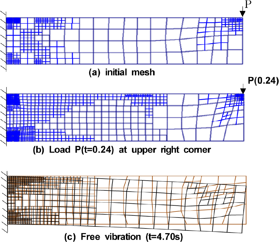
Table 2

Run times and error

Solution	Total Displacement Error % vs Very Fine Mesh Solution	Total Stress Error % vs Very Fine Mesh Solution	Run Time (% vs Engineering Solution)
Very Fine Mesh Solution (6400elements)	0.0% (assumed no error)	0.0% (assumed no error)	5min. 56sec. (266.66% increase)
Engineering Solution (1600elements)	3.592%	2.822%	1min. 48sec. (0.0%)
Strategy Solution (560-826elements)	0.321%	0.221%	42sec. (62.96% decrease)

3.2 Adaptive meshes generated for a portal example

Fig. 5 shows dimensions of a portal frame with a loading P(t) at the top mid point (point B in the figure). The loading P(t) is the same as the one considered in the cantilever example in Section 3.2, i.e., one sinusoid given in Eq. (14) for one second and free vibration for four seconds following. Fig. 6 shows adaptively generated meshes. The mesh generated at t = 0.275 seconds when the vertical deflection of point A is at the maximum is shown in Fig. 6(a). This is during forced vibration and the number of elements is the maximum at 840. Fig. 6(b) shows the mesh where the number of elements is the minimum at 760. This is at t = 3.760 during free vibration.

https://static.apub.kr/journalsite/sites/jcoseik/2024-037-01/N0040370107/images/Figure_jcoseik_37_01_07_F5.jpg

Fig. 5.

Dimensions of portal example

https://static.apub.kr/journalsite/sites/jcoseik/2024-037-01/N0040370107/images/Figure_jcoseik_37_01_07_F6.jpg

Fig. 6.

Generated adaptive meshes for portal example

Stress results from a properly coded finite element program must pass patch test which in simple terms mean ‘constant stress must be exactly reproduced.’ Theoretically, the variations in stress values within an element are the sources of error in the finite element results. Thus a good mesh avoids distorted element shapes and the fineness of mesh is directly proportional to the gradient of stress so that the stress in a given element is close to a constant value. In regions where the stress is expected to be constant or stress free, element sizes may be large and in regions around stress concentration (high stress gradient), the elements must be very fine. In Fig. 6, outer corners of the portal are stress free regions and the generated meshes here have large elements. Inner corners and and under the load areas(see Fig. 6(a)) are stress concentration regions and the meshes are very fine here. The value of stress(largeness) and displacement by themselves are irrelevant in forming a good finite element mesh.

4. Conclusions

Structural analysis automation is an important ingredient of a hazard mitigation system related to architectural and civil structures. For automation, the needed finite element mesh generation scheme for finite element analysis of a structures is presented. The specified procedure for the r-h method based adaptive mesh generation is efficient in terms of real time without any significant decrease in accuracy of the solutions. The algorithm utilizes the commonly known finite element related concepts such as the h-method and the r-method of mesh refinement, shape factors for distortion of element shapes, and strain deviations for estimation of error; the computational time required for incorporating these concepts are small. The case study of a cantilever dynamics example shows specifics of the procedure. The generated adaptive meshes for the portal frame example show the appropriateness of the procedure where the generated fine meshes are shown to be around high stress gradient areas, and coarse meshes are in the constant or zero stress regions. The automation schemes may be used in the structural analysis module in any integrated system or in any part of nonlinear structural analysis and general dynamic analysis of a structure based on the finite element method. The procedure is general enough to be used for real time numerical computation of responses of large complicated structures subjected to real time dependent loads such as earthquakes and extreme weather conditions as efficient and accurate automated analyses of these dynamic and nonlinear problems are becoming an essential part of today’s integrated hazard mitigation systems. The further development of an expert system that produces more powerful initial mesh and use of that expert system to generate more effective initial mesh should improve the performance of automation.

Acknowledgements

This work was supported by 2021 Hongik University Research Fund.

References

Bathe, K.J., Wilson, E.L. (1976) Numerical Methods in Finite Element Analysis, Prentice Hall, Englewood Cliffs.

Belytschko, T., Hughes, J.R., Bathe, K.J. (1996) Finite Element Procedures, Prentice-Hall, Englewood Cliffs.

Jeong, Y.C., Yoon, C. (2003) Representative Strain Value Based Adaptive Mesh Generation for Plane Stress, Hongik J. Sci. & Tech., 7, pp.71~86.

McFee, S., Giannacopoulos, D. (2001) Optimal Discretizations in Adaptive Finite Element Electromagnetics, Int. J. Numer. Meth. Eng., 52(9), pp.939~978. 10.1002/nme.240

Newmark, N.M. (1959) A Method of Computation for Structural Dynamics, J. Eng. Mech. Division, Am. Soc. Civil Eng., 85(EM3), pp.67~94. 10.1061/JMCEA3.0000098

Ohnimus, S., Stein, E., Walhorn, E. (2001) Local Error Estimates of FEM for Displacements and Stresses in Linear Elasticity by Solving Local Neumann Problems, Int. J. Numer. Meth. Eng., 52(7), pp.727~746. 10.1002/nme.228

Yoon, C. (2014) Adaptive Finite Element Mesh Generation for Dynamic Planar Problems, J. Korea Soc. Hazard Mitig., 14(4), pp.43~49. 10.9798/KOSHAM.2014.14.4.43

Yoon, C. (2019) An Automated Adaptive Finite Element Mesh Generation for Dynamics, EESK J. Earthq. Eng., 23(1), pp.83~88. 10.5000/EESK.2019.23.1.083

Yoon, C. (2023) An Automated Adaptive Finite Element Mesh Generation for Dynamics, EESK J. Earthq. Eng., 27(2), pp.77~82. 10.5000/EESK.2023.27.2.077

Zhu, J.Z., Zienkiewicz, O.C., Hinton, E., Wu, J. (1991) A New Approach to the Development of Automatic Quadrilateral Mesh Generation, Int. J. Numer. Meth. Eng., 32, pp.849~866. 10.1002/nme.1620320411

Zienkiewcz, O.C., Zhu, J.Z. (1987) A Simple Error Estimator and Adaptive Procedure for Practical Engineering Analysis, Int. J. Numer. Meth. Eng., 24, pp.337~357. 10.1002/nme.1620240206

Zienkiewicz, O.C., Taylor, R.L., Zhu, J.Z. (2005) The Finite Element Method: Its Basis and Fundamentals, 6th Ed. Elsevier Butterworth-Heinemann, Oxford.

Journal of the Computational Structural Engineering Institute of Korea ISSN:1229-3059(Print) 2287-2302(Online) 한국전산구조공학회 논문집

Preview

Automated Finite Element Analyses for Structural Integrated Systems

ABSTRACT

MAIN

(1)

(2)

(3)

(4)

(5)

(6)

(7)

(8)

(9)

(10)

(11)

(12)

(13)

(14)

Fig. 1.

Cantilever beam and loading P(t)

Table 1

A Progression of strain deviation values

Fig. 2.

Automatically generated finite element meshes for cantilever example

Fig. 3.

Uniform mesh commonly used (cantilever example)

Fig. 4.

Comparisons of displacement and stress solutions

Table 2

Run times and error

Fig. 5.

Dimensions of portal example

Fig. 6.

Generated adaptive meshes for portal example

Acknowledgements

References