

1. Introduction
The hydrodynamic pressure acting on dam and other submerged hydraulic structures during earthquake plays an important role in the analysis and design. It has been widely and frequently investigated by many researchers because of its important and direct application in designing a dam. Significant research has been devoted to this subject since the first study of Westergaard(1933) who modeled hydrodynamic forces as an added mass attached to the upstream face of dams. Although Westergaard’s analytical formulation was developed assuming rigid dam impounding incompressible water, it has been widely used for many decades to design earthquake-resistant concrete dams thanks to its simplicity(USACE, 2007;USBR, 2006). For a dam whose upstream face is not vertical, Zangar(1952) determined the hydrodynamic pressure experimentally using an electrical analogue. Chwang (1978) presented approximated solutions obtained from the momentum balance principle for the hydrodynamic pressure distribution acting on an inclined dam face. It was assumed that the duration of the dam acceleration is short enough so that the compressibility of the fluid is negligible. During the last four decades, several researchers developed advanced analytical and numerical approaches to account for dam deformability and water compressibility in the seismic response of concrete dams(Chopra, 1970;Chakrabarti and Chopra, 1973;Chopra, 1978;Saini et al., 1978;Hall and Chopra, 1982;Fenves and Chopra, 1984;Pelecanos et al., 2016).
However, all the above studies were based on the assumption of water surface remaining constant and horizontal during earthquakes, and this assumption was valid when the instantaneous ground displacement was small. The rise of the free surface and the nonlinear convective acceleration were first included in Chwang's(1983) analysis with a rigid vertical wall and constant ground acceleration. Chen(1994, 1996), using a two-dimensional finite difference scheme, studied the variation of the water surface and the corresponding nonlinear hydrodynamic pressures acting on rigid (or deformable) dam faces with various reservoir shapes. Chen et al.(1999) extended the research to the three-dimensional hydrodynamic pressure analysis. Chen and Yuan(2011) developed a complete threedimensional finite difference scheme to analyze the nonlinear hydrodynamic pressures on arch dams during earthquakes. Both free-surface waves and nonlinear convective acceleration are included in the analysis. While those theoretical and numerical studies have been focused on vertical, inclined or slightly-curved faces of a dam, hydrodynamic pressure applying to a radial gate has not been investigated sufficiently and the Westergaard added mass concept is still widely used(USACE, 2000;USACE, 2007;USBR, 2006), which is not accurate and appropriate for large radial gate structures.
In this study, a computational approach for structurereservoir interaction systems is suggested to realistically simulate the hydrodynamic pressures on dams and radial gates during strong earthquakes based on the Arbitrary Lagrangian-Eulerian(ALE) approach(Hirt et al., 1974;Donea et al., 1982). The structural face subjected to hydrodynamic pressure is modeled as a moving boundary interacting with the reservoir during earthquake excitation. To implement the ALE and free reservoir surface model, functions from a generalpurpose fluid dynamics software is used with newly composed interface program to transfer structural deformation caused by earthquake ground motions. The suggested model approach is verified and validated by comparing hydrodynamic pressures from the earthquake simulation with ones obtained by Wetergaard's formulation for vertical dam faces and Zangar’s formulation for vertical and inclined structural faces. A parameter study for truncated lengths of the twodimensional fluid domain is performed to determine the numerically appropriate distance to transmitting boundary conditions at the upstream end of the reservoir model. Lastly, numerical results of hydrodynamic pressure are presented for different curvature shapes of the large radial gate to validate the suggested approach.
2. Computational model
2.1 Reservoir model
In the present study, it is suggested to use a moving mesh to model a reservoir domain with moving boundaries due to strong earthquakes, since the strong ground motions can cause significant interface movement and consequently, large change of the domain. Moving mesh can be considered by the ALE formulation, which makes it possible to include grid velocities in the momentum and the continuity equations, as shown below:
where t is the time, ρ is the fluid density, υ is the flow velocity vector, υg is the mesh velocity of the moving mesh, p is the pressure, τ is the viscous stress tensor, and n is the normal vector. Here ∂Ω is used to represent the boundary of the control volume Ω.
For the convection terms in Eq. (1), a second-order upwind scheme is used to interpolate the face values of various quantities from cell centre values. The diffusion terms are central differenced and secondorder accurate. The temporal discretization process is carried out using a first order implicit scheme. The SIMPLE algorithm(Patankar and Spalding, 1972) is used to relate the pressure to the velocity. The discretized equations are then solved sequentially using a segregated solver.
The treatment of free surface flow for the reservoir is performed by using the Volume-of-Fluid(VOF) method(Hirt and Nichols, 1981;Phan and Lee, 2010). The tracking of the interface(s) between the phases is accomplished by the solution of a continuity equation for the qth volume fraction parameter, αq . For the qth phase, where ρq is the fluid density and υq is the flow velocity vector, this equation has the following form:
where is the mass transfer from phase p to phase q and is the mass transfer from phase q to phase p.
In the present study, the explicit scheme for the discretization of volume fraction function is selected. The geometric reconstruction approach(Youngs, 1982;Rider and Kothe, 1998) which represents the interface between fluids using a piecewise-linear approach is used to obtain the face fluxes whenever a cell is completely filled with one phase or another.
2.2 Structure-reservoir interaction during earthquake excitation
In the present computational model, an earthquake ground motion is simulated as moving boundaries of a fluid reservoir domain as shown in Fig. 1. The deformation and rigid-body motions of a structure due to a ground acceleration is numerically solved over time domain. Through the newly composed time integration module, at the end of each time step, the ground acceleration applied to the dam is passed as the boundary changes for a reservoir domain. Then the new geometry configuration is applied to the fluid domain and the ALE algorithm updates the finite volume mesh associated with the moving boundary (Fig. 1).
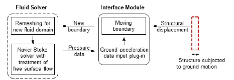
The dynamic layering method(ANSYS, 2010) is used to add or remove layers of cells adjacent to the moving boundary. In this method, the layer of cells adjacent to the moving boundary is split or merged with the layer of cells next to it based on the width of the next layer. This technique allows a much smaller computational time than other dynamic remeshing ones, e.g., smoothing or local remeshing methods.
3. Model verification and validation tests
To implement the computational model approach suggested in this study, the ALE and free water surface algorithm functions in FLUENT(ANSYS, 2010) is used for reservoir domain, with a newly composed module written in the user-defined function, which can be dynamically loaded with the FLUENT solver to transfer earthquake ground motions through a structure at each time step. The reservoir simulation with free surface is based on the Navier-Stokes equations which describe the motion of an incompressible viscous fluid flow. The density and viscosity of the water reservoir are 998.2kg/m3 and 0.001003kg/(m·s), respectively.
3.1 Earthquake ground motions
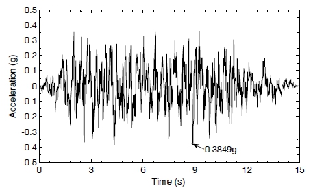
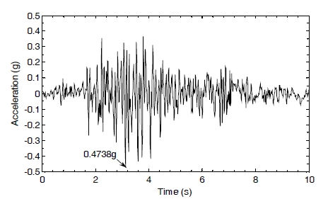
To investigate the dam-reservoir interaction subjected to strong earthquake loadings, the horizontal components of an artificial ground motion and Koyna ground motion are selected. The time history of these ground motions are given in Fig. 2 and Fig. 3 with a time step, Δt = 0.01s.
3.2 Hydrodynamic pressure on vertical dam surfaces
Several two-dimension numerical simulations of the dam-reservoir interaction are presented to verify the accuracy and demonstrate the capability of the present work. The hydrodynamic pressure distributions developed due to artificial ground motion along the dam-reservoir interface are evaluated and compared with Zangar’s experiment formulation(1952) and Westergaard’s analytical formulation(1933). For comparison purposes, the dam structure is assumed to be rigid.
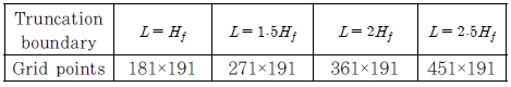
In the first example, the upstream face of the dam is considered to be vertical and the bottom of reservoir to be horizontal. Fig. 4 shows a schematic of damreservoir system with vertical surface of upstream face. The depth of the reservoir Hf is considered to be 72m. The effectiveness of the reservoir length is examined for four different transmitting boundary condition locations: L = Hf , 1.5Hf , 2Hf , and 2.5Hf .
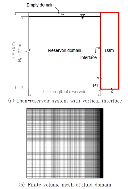
In the present parametric study, a none-uniform grid of fluid domain is used considering the quadrilateral control volumes. The number of grid points for the four locations of truncation boundary is shown in Table 1. All the results of pressure distribution are obtained in terms of the hydrodynamic pressure coefficient, cp, defined by:
where p is the hydrodynamic pressure; ρ is the unit mass of water; and a is the Peak Ground Acceleration (PGA).
Fig. 5 shows the contours of dam-reservoir interaction with free surface motion. The peak values of hydrodynamic pressure on the vertical upstream face of dam with different truncated boundary locations are shown in Fig. 6. As observed in the figure, the results for far truncated boundary locations L = 2Hf and L = 2.5Hf are almost the same, while that of truncated boundary L = Hf gives remarkably bigger pressures.
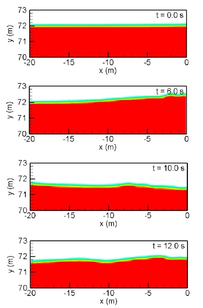
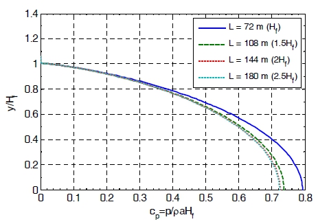
Fig. 6
Peak value of hydrodynamic pressure acting on vertical upstream face of dam with different reservoir lengths
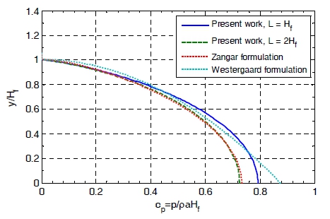
In Fig. 7, the results obtained for two cases of truncated boundary L = Hf and L = 2Hf are compared with the results obtained by Westergaard and Zangar formulations. Here, y represents the vertical distance from the bottom of the reservoir. Overall, the present work shows more realistic results than those obtained by Westergaard’s formulation(USBR, 2006). When the short distance of truncated boundary L = Hf is considered, the discordance between the present model and the Zangar’s formulation is apparent. However, the agreement between two methods is excellent for reservoir with far truncated boundary locations, L = 2 Hf and L = 2.5Hf. It can be concluded that the truncated boundary located at L = 2Hf gives the efficient and still converged results compared with the other locations.
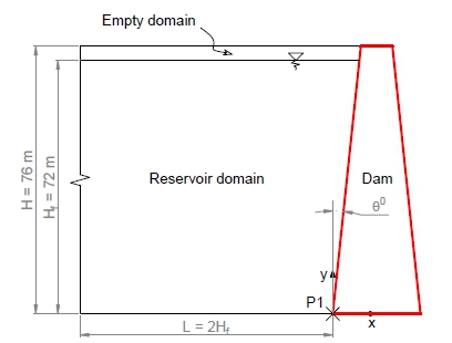
3.3 Hydrodynamic pressure on inclined dam surfaces
In this section, the hydrodynamic pressure distributions along the dam-reservoir interface with different inclinations of the upstream face are presented. Fig. 8 shows a schematic of dam-reservoir system with sloping interface. To verify and compare the numerical results with the Zangar formulation, the dam is assumed to be rigid. Similar to the previous example, the depth of reservoir, Hf , is 72m and the length is taken as 2Hf as chosen in Section 3.2.
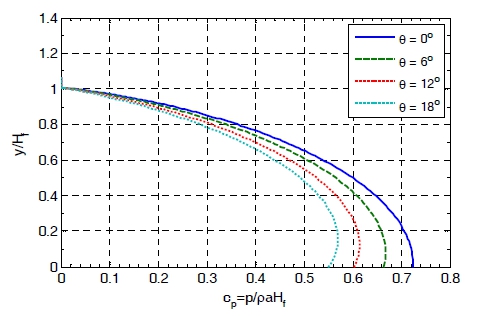
The effect of the upstream shape on the pressure distribution is observed in Fig. 9 for dam with different sloping faces. The hydrodynamic pressure coefficient is calculated for the cases of θ = 0°, 6°, 12° and 18°. It can be seen that the largest and smallest values of hydrodynamic pressure are generated for the cases of vertical (θ = 0°) and fully inclined (θ = 18°) surface, respectively.
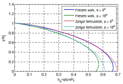
The results obtained for truncated boundary location, L = 2Hf , and sloping angles, θ = 6° and θ = 18°, are compared in Fig. 10 with the results obtained by Zangar’s formulation. The agreement between the present results is very good except close to the bottom for high-sloping angles. Considering the original experimental data by Zangar(1952;USBR, 2006) rather than its simplified formulation used for plotting in Fig. 10, the agreement becomes much better, which shows the validation of the suggested computational model.
4. Numerical simulation for hydrodynamic pressure on radial gates
The validation example considered in this section is for radial gate structures subjected to two strong ground motions: artificial ground motion and Koyna ground motion. The geometries of the reservoir fluid domain and radial gate structure interface are shown in Fig. 11. The radial gate with 20m height is considered with different curved surfaces. The water level of the reservoir at initial time, Hf , is 18m and the truncated boundary location, L = 2Hf , is proposed in this example. Fig. 12 shows the variation of the hydrodynamic pressure at the base as the time is varied from 3 to 9 sec.
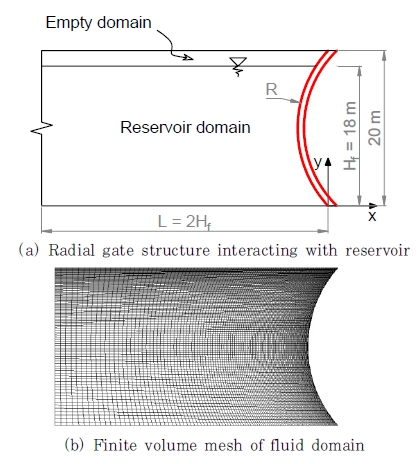
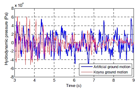
Fig. 12
Time history data of hydrodynamic pressure acting at the bottom of radial gate with surface curvature R=18 m subjected to two kinds of ground motion
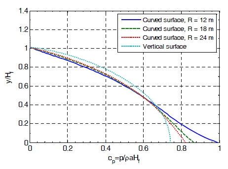
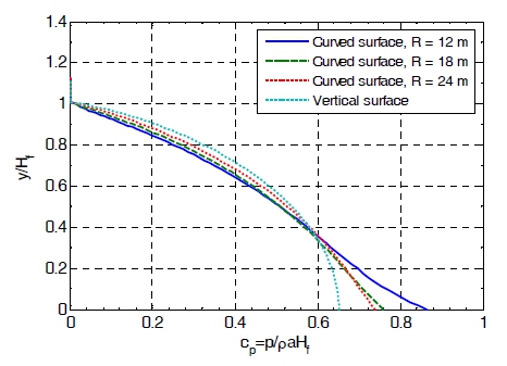
Hydrodynamic pressure distributions acting on the structure-reservoir interfaces are shown in Fig. 13 and Fig. 14. The upstream face with different curvatures, R=12m, 18m, and 24m, are considered to estimate the effect of curved surfaces on the hydrodynamic distribution. The hydrodynamic coefficient corresponding to the radial gate with vertical surface is also plotted. It can be seen from the figures, the radius of radial gate surface does not significantly influence to the hydrodynamic pressure distributions in 0~60% of the water level from the surface. On the contrary, the radial gate with the largest curvature (R=12m) shows the highest value of hydrodynamic pressure than those with smaller ones and vertical surface near the bottom range, in 60~100% of the water level from the surface. The hydrodynamic pressure at the bottom of the largest curvature radial gate is approximately 33% higher than the vertical one for both the artificial and Koyna earthquakes.
5. Conclusion
A computational model approach for nonlinear hydrodynamic pressures acting on radial gates during strong earthquakes has been presented. It is suggested to use the dynamic layering method with ALE algorithm and the SIMPLE method for simulating free reservoir surface flow. The verification and validation of the proposed approach has been successfully realized by the comparisons performed using the renowned formulation derived by experimental results for vertical and inclined dam surfaces subjected to earthquake excitation. A parameter study for truncated lengths of the two-dimensional fluid domain shows that two times the water level provides the numerically appropriate distance to transmitting boundary conditions at the upstream end of the reservoir model, which gives the efficient and converged results. Numerical simulations for large radial gates with different curvatures subjected to two strong earthquakes have been successfully performed using the suggested computational model. The results show the hydrodynamic pressure at the bottom of the largest curvature radial gate is approximately 33% higher than the vertical one for both the artificial and Koyna earthquakes. It is concluded that the appropriate fluid-structure interaction computational model rather than the Westergaard added mass model needs to be used in analysis and design for large radial gates subjected to strong earthquake excitation.
