

1. Introduction
Social vulnerability is difficult to quantify, therefore Cutter et al. (2003) proposed the construction of Social Vulnerability Index (SoVI) as a basis for local officials, emergency managers, and planners to add to their action plan on disaster response in order to allocate the necessary resources in the events of disasters to the right targets at the right location (Cutter et al., 2003; UCHSC, 2004; Boruff et al., 2005; Boruff et al., 2007).
The similar study also conducted by the work of Pungky Utami (2009) with unit of analysis in village district and analysis census-based data without a qualitative survey based-data. However, this study carried out analysis on the level of hamlet, instead of village district, since a village may be located in several hazard zones (observation by Sagala and Okada). Also, social vulnerability captured here is using a qualitative survey based-data such as interviews to local people and stakeholders to help define social vulnerability variables by conducted fieldwork which consisted of one and a half weeks during September 2-11, 2013. It was covering of two trips, first was surveyed the environment and residential building and interviews to the local people in Turgo and Kaliurang Barat hamlet, Pakem District, Sleman Regency related to vulnerability. Second, interviews and collecting data from stakeholders such as BPPTKG, Yogyakarta and BPBD Sleman (Regional Disaster Management Board).
2. Case Study Area
According to Suryo and Clarke (1985), the most common hazards following a volcanic eruption in Indonesia are lava flows, volcanic blocks and bombs, pyroclastic flows, lahars, and ash plumes, which commonly occur in Merapi volcano. Merapi has high volcanic activity and it is the most active of least 129 active volcanoes in Indonesia, located in Java Island which has been responsible for thousands of deaths in the region. Since AD 1000, Merapi has erupted more than 80 times. Merapi eruption in 2010 was the biggest (VEI 4), compared with the same disaster in five occurrences in the past 1994, 1997, 1998, 2001, 2006 and caused death loss around 400 people.
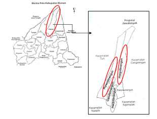
The focus of this study was in Turgo hamlet in Purwobinangun village and Kaliurang Barat hamlet in Hargobinangun village, Pakem District, Sleman Regency, Special Region of Yogyakarta, as shown in Fig. 1. The study areas are involved as Hazard Zone III (KRB III). Hazard Zone III is a disaster-prone areas often pounded by hot clouds, lava flows (avalanches /burst of incandescent material), toxic gases.
3. Social Vulnerability Index (SoVI) Analysis
The study runs Statistical Package for Social Science (SPSS) to process the data set and using Principal Component Analysis (PCA) analysis.
Tabachnick and Fidell (2007) explained several steps in running PCA, which include selecting a set of variables, preparing correlation matrix, extracting a set of components from the correlation matrix, determining the number of components to extract by Kaiser’s criterion as well as scree plot, rotating the components to increase its interpretability, and interpreting the results.
In the early stage, the calculation for this study was only for two hamlets as case study i.e. Turgo and Kaliurang Barat hamlets. The initial dataset for those two cases study were proved invalid as the number of cases was less than the number of variables, thus PCA would not produce reliable results. Due to that reason, other hamlets were added to perform the calculation, which using the statistical data obtained from the website of Sleman Regency statistical office.
Statistical identification is very important in terms of engineering field (Yang et al., 1993). In this case, the statistical data obtained from Pakem District in Figures 2007 and Sleman Regency in Figures 2010. Due to the limited and availability of data, the assumption was taken in this study. The unit analysis in this study was at the hamlet level; therefore all indicators in this research were then calculated at the hamlet level. Data obtained were derived and adjusted according to the amount of population in each hamlet to get numbers in statistical data in the level of hamlet.
The vulnerability index is constructed from nine socio-economic concepts which collectively represent a universal concept of social vulnerability. A Principal Component Analysis (PCA) is used to reduce the number of variables into fewer components that are uncorrelated with all others (Lattin et al., 2003). After observing the vulnerability variables relevant to the case study, there were 14 variables (Table 1) available for further analysis.
The research identifies the underlying factors which increase the social vulnerability by assessing the variables used to measure social vulnerability. To obtain the SoVI, two steps of analyses will be carried out. The first step is variable reduction and then followed by the calculation of social vulnerability index, as explained in the following section.
Table 1
Social vulnerability variables, concepts and rationale
3.1 Variable reduction
The Principle Component Analysis was taken to reduce correlated variables into several uncorrelated appropriate components using varimax rotation and the eigenvalues greater than 1. The component which has eigenvalues greater than 1 will extract, and then used to measure the social vulnerability of each hamlet. The statistical steps explained as following section.
Because of the value and unit of each variable is different, then the raw data need to be performed using data standardization Z-score. Z-scores are expressed in terms of standard deviations from their means. Resultantly, these z-scores have a distribution with a mean of 0 and a standard deviation of 1. The formula for calculating the standard score is given below
Where μ is mean, X is score, and σ is standard deviation. The value of z is positive when the value is greater than the mean, and z is negative when the value is less than the mean.
For the Kaiser-Meyer-Olkin (KMO) Measure of Sampling Adequacy (MSA) presented in Table 2 tests that the partial correlation among variables are small. KMO’s statistic Kaiser (1974) recommends a bare minimum of 0.5 and that values between 0.5 and 0.7 are mediocre, values between 0.7 and 0.8 are good, values between 0.8 and 0.9 are great and values above 0.9 are superb (Hutcheson et al., 1999). For any variables with values below 0.5 then it should consider excluding from the analysis and repeat the analysis without them. The KMO’s equation is,
Table 2
KMO and Bartlett’s test
| Kaiser-Meyer-Olkin Measure of Sampling Adequacy | 0.804 | |
|---|---|---|
| Bartlett’s Test of Sphericity | Approx. Chi-Square | 330.813 |
| df | 66 | |
| Sig. | 0.000 | |
Where  is coefficient of simple correlation between variable
  and
and  , and
, and  is coefficient of partial correlation between variable
  and
and  . Measure of Sampling Adequacy (MSA) equation is,
Bartletts test of sphericity measure tests the null hypothesis that the original correlation matrix is an identity matrix. A significant test tells us that the R-matrix is not an identity matrix; therefore, there are some relationships between the variables we hope to include in the analysis. For these data, Bartlett’s test is highly significant if p < 0.001. The Bartletts’s equation is,
Where N is the amount of observation, p is the amount of variable and |R| is determinant matrix correlation.
According to the process calculation as explained in above steps, the two variables i.e. POPDNSTY and AGRCLTR have to be removed because do not meet the requirements. After removing POPDNSTY and AGRCLTR variables, it shows from the results in Table 2, the KMO value is 0.804; means the value is great since correlations between pairs of variables can be explained by the other variables. Bartlett’s test is 0.000, means highly significant if p <0.001. Hence, the samples could be analyzed further without AGRCLTR and POPDNSTY variables.
In this calculation, the result of Measure of Adequacy Sampling (MSA) for all variables is more than 0.5, then it can be analysed further. Only those with eigenvalues >1 (Kaiser criterion, Kaiser 1960) which need to be considered. As factors with eigenvalues <1 can be said to be not significant, as shown in Table 3.
Table 3
Initial Solution
Extraction Method: Principal Component Analysis
An eigenvalue represents the amount of variance accounted for by a factor. Because the variance that each standardized variable contributes to a principal factor extraction is 1, a factor with an eigenvalues less than 1 is not as important, from a variance perspective, as an observed variable. Variance factor is formed of the % of Variance on Extraction Sums of Squared Loadings.
An extraction procedure is usually accompanied by rotation to improve the interpretability and scientific utility of the solution. The purpose of rotation is to achieve a simple structure in which each factor has large loadings in absolute value for only some of the variables, making it easier to identify (Nourusis, 2003). In this case, choose the most common orthogonal rotation method known as varimax was developed by Kaiser (1958).
For varimax a simple solution means that each factor has a small number of large loadings and a large number of zero (or small) loadings. This simplifies the interpretation because after varimax rotation, each original variable tends to be associated with one (or a small number) of factors, and each factor represents only a small number of variables.
Where  being the squared loading of the
  variable on the
  factor and
  being the mean of the squared loadings.
Following in the Table 4 are derived components which are used to construct the social vulnerability index for each hamlet. Factor with the greatest values are classified into Factor 1 with variance on extraction sums of square loadings is 66.659% and Factor 2 is 14.866%.
Table 4
Component and loading used to construct the social vulnerability index
3.2 Calculation of Social Vulnerability Index (SoVI)
The next step is derived the components which are used to construct the social vulnerability index for each hamlet. The total components’ score is summed to create the social vulnerability index score. The score is classified into levels ranging from the value < -1.5 indicating low social vulnerability to the value > +1.5 indicating high social vulnerability.
From the results of PCA analysis, factor score values obtained for each hamlet and the factor 1 score and factor 2 score are summed to create the total social vulnerability index score (SV score), shown in Table 5.
Table 5
Ranking of Social Vulnerability Index (SoVI)
 Pakem District
 Kalasan District
 Tempel District
As the case study in Pakem District, Turgo hamlet has - 0.53 score and Kaliurang Barat hamlet has - 0.56. It means that Turgo hamlet is more vulnerable than Kaliurang Barat hamlet. It is also shown that Juwangan hamlet in Kalasan District with 3.75 score is the most vulnerable than others.
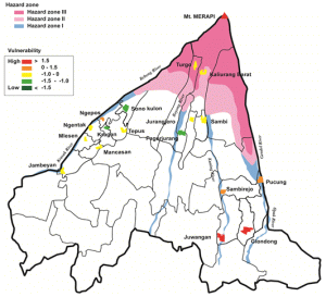
The next step is to map the social vulnerability score derived from the statistical analysis. The social vulnerability map and the Merapi’s volcanic hazard map 2010 (BPPTK) are overlaid together. According to the social vulnerability map in Fig. 2, the finding is that the high socially vulnerable people do not necessarily reside within hazard zone III or II, taking the example of Juwangan and Glondong hamlets reside within hazard zone I that has highest socially vulnerable than others where these two hamlets located near the river. Juwangan hamlet located near to Kuning River and Glondong hamlet located near to Opak River.
3.3 Dominant influence of individual variables
In order to predict which individual variables give significant contributions to the total score, the study applies the stepwise regression method. The standardized beta coefficients in the stepwise regression indicate the strength independent variables (vulnerability variables) with the dependent variable (social vulnerability score). As shown the result in Table 6, shows the number of vehicle non-motorized is the most important contributor of social vulnerability in all hamlets. According to the result of interviews with the people in study area, transport was the initial list of vulnerability variable that most frequently mentioned as they are lack of transportation, since they need quick access during evacuation. The result is followed by the families’ number and the number of unemployment.
Table 6
Dominant social vulnerability variables rank based on standardized beta coefficient(β)
| Standardized variables | β | Sig.(<0.05) |
|---|---|---|
| Number of vehicle non-motorized | 0.461 | 0.000 |
| Families number | 0.412 | 0.000 |
| Number of unemployment | 0.232 | 0.001 |
The removed variables shown in Table 7 which are grouped in a separate table below show that their significance values (Sig.) do not meet the requirement (< 0.05), therefore the hypothesis that the variables do not demonstrate strong relationship with the dependent variable is accepted. To interpret the results, only the first few columns are relevant to this study, namely the beta value (Beta In), t-statistic (t) and the significance value (Sig.). The beta value and t-statistics show the degree to which each predictor affects results if the effects of other predictors are held constant (Field, 2005).
Table 7
Exclude variables
a. Predictors in the Model:(Constant), Zscore(VEHCNNMT)
b. Predictors in the Model:(Constant), Zscore(VEHCNNMT), Zscore(FAMNUMB)
c. Predictors in the Model:(Constant), Zscore(VEHCNNMT), Zscore(FAMNUMB), Zscore(EMPLYLS)
d. Dependent Variable: totsovi
4. Conclusion
The creation of vulnerability index is a useful starting point when trying to capture vulnerability. This approach depends much on the quality, availability of the data and the unit of analysis that are dealing with. This study carried out analysis on the level of hamlet, instead of village district, since a village may be located in several hazard zones. The finding from the analysis using SoVI confirms that this method works well in ensuring that positive values indicating high social vulnerability and vice versa. The small number of cases has created few difficulties in processing the dataset since PCA requires large sample size. In addition, according to the interviews to the local people, found that experiences of disaster in the past eruption might make the people more prepared for future scenarios. Most interviewees understand that children, baby, elderly, pregnant mother are the most vulnerable group. Most people in both study areas have a good understanding of the dangers of volcano, as they received education and socialization from government such as BPPTKG and BPBD Sleman.
