Quasi-brittle and Brittle Fracture Simulation Using Phase-field Method based on Cell-based Smoothed Finite Element Method

Changkye Lee; Sundararajan Natarajan; Jurng-Jae Yee

doi:10.7734/COSEIK.2023.36.5.295

Preview

Research Paper

Journal of the Computational Structural Engineering Institute of Korea. 31 October 2023. 295-305
https://doi.org/10.7734/COSEIK.2023.36.5.295

Quasi-brittle and Brittle Fracture Simulation Using Phase-field Method based on Cell-based Smoothed Finite Element Method

셀기반 평활화 유한요소법에 기반한 위상분야법을 이용한 준취성 및 취성 파괴 시뮬레이션

Changkye Lee¹

Sundararajan Natarajan²

Jurng-Jae Yee³^*

이 창계¹

Sundararajan Natarajan²

이 정재³^*

¹Senior Researcher, University Core Research Center for Disaster-free & Safe Ocean City Construction, Dong-A University, Busan, 49315, Korea

²Professor, Department of Mechanical Engineering, Indian Institute of Technology Madras, Chennai, 600036, India

³Professor, Department of Architectural Engineering, Dong-A University, Busan, 49315, Korea

¹동아대학교 해양도시건설･방재연구소 선임연구원

²인도마드라스공과대학 기계공학과 교수

³동아대학교 건축공학과 교수

^{*Corresponding Author}

ABSTRACT

This study introduces a smoothed finite-element implementation into the phase-field framework. In recent years, the phase-field method has recieved considerable attention in crack initiation and propagation since the method needs no further treatment to express the crack growth path. In the phase-field method, high strain-energy accuracy is needed to capture the complex crack growth path; thus, it is obtained in the framework of the smoothed finite-element method. The salient feature of the smoothed finite-element method is that the finite element cells are divided into sub-cells and each sub-cell is rebuilt as a smoothing domain where smoothed strain energy is calculated. An adaptive quadtree refinement is also employed in the present framework to avoid the computational burden. Numerical experiments are performed to investigate the performance of the proposed approach, compared with that of the finite-element method and the reference solutions.

Keywords

phase-field method

smoothed finite element method

quadtree refinement

crack propagation

본 연구에서는 평활화 유한요소법(Smoothed finite element method)을 도입한 위상분야법(Phase-field method)에 대해 소개하고자 한다. 위상분야법은 최근 균열 개시 및 전파 해석에 많이 사용되는 기법으로 균열 표면을 추적하기 위한 추가적인 처리기법이 필요하지 않는 특징이 있다. 위상분야법에서 복잡한 균열 전파를 포착하기 위해 높은 정확도의 변형률 에너지를 평활화 유한요소법을 도입하여 계산하였다. 평활화 유한요소법은 유한요소를 하위 셀로 나누고 각각의 하위 셀을 평활화 영역으로 재조립하여 변형률 에너지를 계산하게 된다. 또한 해석 시간 단축을 위하여 쿼드트리 요소망을 제안한 기법에 사용하였다. 수치 예제를 통하여 제안한 기법을 참조해 및 유한요소법과 비교하여 검증하였다.

키워드

위상분야법

평활화 유한요소법

쿼드트리 요소망

균열 전파

MAIN

1. Introduction
2. Theoretical Background of Phase-field Method
3. Smoothed Finite Element Method: Overview
3.1 Quadtree refinement
3.2 Wachspress basis functions
4. Numerical Tests
4.1 Cantilever beam
4.2 Patch test
4.3 Plate with the crack
5. Conclusion

1. Introduction

The fracture mechanism is one of the critical matters in modern engineering applications. In particular, the prediction of initiation and propagation of the crack path is a dominant concern for engineers and scientists. Therefore, to treat such obstacles, various numerical attempts, viz. discontinuous and continuous methods, have been suggested (Zhuang et al., 2022). Well-known discontinuous approaches are the extended finite element method (X-FEM) (Moës and Belytschko, 2002; Yoo and Kim, 2016) and generalized finite element method (GFEM) (Fries and Belytschko, 2010). Typically, these approaches utilize further schemes to handle crack tip singularity. Although this leads to improved accuracy, the numerical implementation often suffers from its mathematical complexity. In recent years, one of the continuous approaches, i.e., phase-field method (Miehe et al., 2010a; 2010b), has caught researchers’ interest. The phase- field possesses notable characteristics, including modeling the crack as a geometric discontinuity while treating the cracked domain as a continuum. Thus, additional treatment for crack initiation is not required. In addition, it has been instrumental in commercial/academic software (Hirshikesh et al., 2018; Molnár and Gravouil, 2017). Notwithstanding its ease of implementation, the phase-field method encounters a computational burden as the discontinuity evolves over time (Hirshikesh et al., 2018). Accordingly, quadtree mesh refinement can be a practical candidate to save mesh generation labor (Finkel and Bentley, 1974).

In this study, we explore the possibility of incorporating quadtree decomposition and strain smoothing approximations to embrace computational efficiency and accuracy. Since strain smoothing approximation, often called Smoothed Finite Element Method (S-FEM), was introduced by Liu et al. (2007a), the method has shown its tolerance to locking and mesh distortion (Zeng and Liu, 2018). Besides such aspects, S-FEM, in general, shows fast convergence and yields high accuracy in engineering problems (Lee et al., 2022; Liu et al., 2007b) and discontinuity (Bordas et al., 2010; Surendran et al., 2017). In the phase-field framework, highly accurate strain energy density needs to be computed to capture the complex crack growth path. In the S-FEM framework, finite element cells are sub-divided into sub-cells, and then sub-cells are reconstructed as a smoothing domain where gradients are smoothed. The strain energy is also computed on each smoothing domain by the smoothed strains and generally shows an improvement in accuracy (Liu and Nguyen, 2010). Therefore, S-FEM is workably able to bring a reliable crack path in the phase-field method.

The rest of this paper is organized as follows: Section 2 revisits the background of the phase-field method and the overview of S-FEM discussed in the following section. The validation and reliability of the adaptive S-FEM implementation into the phase-field are studied in Section 4 and then major discussion is drawn in the last section.

2. Theoretical Background of Phase-field Method

The basic idea of the phase-field fracture theory is based on the energy theory introduced by Griffith (1921). However, it has a limitation to explain crack growth behavior since the crack initiation and bifurcation are not considered. Hence, Francfort and Marigo (1998) proposed the variational fracture theory using energy-minimizing approximation. The internal energy of the system is given as:

(1)

W = \int_{Ω} Ψ (ε) d Ω + \int_{Γ} G_{c} d Γ

where $G_{c}$ is the critical energy release rate and 𝛹 is strain energy density under the undamaged condition is given by Eq. (2):

(2)

Ψ (ε) = \frac{1}{2} λ (t r (ε))^{2} + μ (ε : ε) = \frac{1}{2} λ (t r (ε))^{2} + μ t r (ε^{2})

where Lame’s first parameter 𝜆 and the shear modulus 𝜇 are computed respectively in terms of Young’s modulus $E$ and Poisson’s ratio 𝜐 as follows: $λ = \frac{E ν}{(1 + ν) (1 - 2 ν)}$ and $μ = \frac{E}{2 (1 + ν)}$ . To numerically solve Eq. (1), a diffused field variable 𝜙 was introduced by Bourdin et al. (2000) to characterize the crack surface as shown in Fig. 1.

https://cdn.apub.kr/journalsite/sites/jcoseik/2023-036-05/N0040360502/images/Figure_jcoseik_36_05_02_F1.jpg

Fig. 1.

Solid body with crack topology

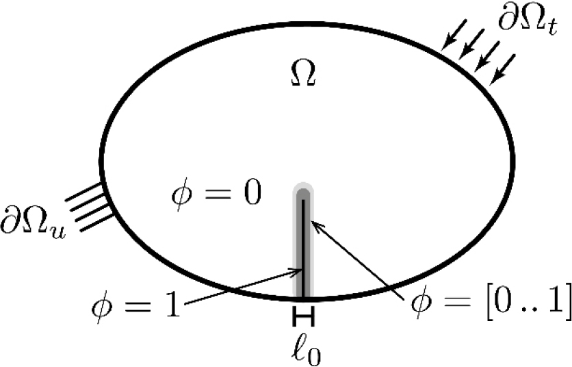
In the phase-field method, the diffused field variable represents the state of the material, i.e., 𝜙=0 represents an undamaged state and 𝜙=1 represents a fully damaged state. The approximation of the fracture energy by the crack can be defined as:

(3)

\int_{Γ} G_{c} d Γ \approx \int_{Ω} G_{c} Γ_{l_{0}} (l_{0}, ϕ) d Ω = \int_{Γ} G_{c} (x) (\frac{1}{2 l_{0}} ϕ^{2} + \frac{l_{0}}{2} | \nabla ϕ |^{2}) d Ω

By substituting Eq. (3) into Eq. (1), we can obtain the energy of the system using Eq. (4):

(4)

W = \int_{Ω} ((1 - ϕ)^{2} Ψ (ε) + G_{c} (\frac{1}{2 l_{0}} ϕ^{2} + \frac{l_{0}}{2} | \nabla ϕ |^{2})) d Ω

where (1-𝜙)² denotes the degradation of the stored energy with evolving damage. Note that, in the framework of the phase- field method, the size of the regularized crack surface is controlled by the internal length scale $l_{0}$ .

By employing Gauss divergence theorem to Eq. (3), the following coupled field equations can be obtained:

(5a)

(1 - ϕ)^{2} \nabla ･ σ = 0 in Ω

(5b)

G_{c} (\frac{1}{l_{0}} ϕ + l_{0} ∆ ϕ) - 2 (1 - ϕ) Ψ (ε) = 0 in Ω

where 𝜎 in Eq. (5a) is the Cauchy stress tensor and the natural boundary conditions are defined in Eqs. (6a) and (6b) as follows, respectively:

(6a)

(1 - ϕ)^{2} σ ･ n = T on Γ

(6b)

\nabla ϕ ･ n = 0 on Γ

In this study, the smoothed finite element approximation is utilized to solve coupled field equations of Eq. (3). To reduce irreversibility, Ambati et al. (2014) proposed a hybrid formulation, as implemented in Eq. (5b), which can be rewritten as Eq. (7):

(7)

G_{c} (\frac{1}{l_{0}} ϕ + l_{0} ∆ ϕ) - 2 (1 - ϕ) H^{+} (ε) = 0

where a historical variable $H^{+}$ , as defined in Eq. (8), was introduced by Miehe et al. (2010a):

(8)

H^{+} = \max_{t \in [0, τ]} Ψ^{+} (ε (t))

where $Ψ^{+} (ε) = \frac{1}{2} K < t r (ε) >_{+}^{2} + μ (ε^{d e v} : ε^{d e v})$ with $< ･ >_{+} = \frac{1}{2} (a + | a |)$ and $K$ is the bulk modulus (Amor et al., 2009).

Applying the standard Bubnov-Galerkin approximation, we can obtain the following weak form of Eq. (10): Find $u \in U$ and $ϕ \in P$ such that, for all $ν \in V^{0}$ and $q \in Q$ ,

(9a)

a (u, v) = l (v)

(9b)

b (ϕ, q) = l (q)

where

(10a)

a (u, v) = \int_{Ω} \{[(1 - ϕ)^{2} + k] σ (u) : ε (v)\} d Ω

(10b)

l (v) = \int_{Ω} b ･ v d Ω + \int_{Γ^{t}} \bar{t} ･ v d Ω

(10c)

b (ϕ, q) = \int_{Ω} \{\nabla q ･ \nabla ϕ G_{c} l_{0} + q (\frac{G_{c}}{l_{0}} + 2 H^{+}) ϕ\} d Ω

(10d)

l (q) = \int_{Ω} 2 H^{+} q d Ω + \int_{Γ} \nabla ϕ ･ n d Γ

where $k$ is a very small value for numerical consistency. To solve Eq. (10), a staggered approach is used, i.e., firstly, the phase field 𝜙 is solved by the displacement fields. Then the phase field is used to solve for the displacement fields.

3. Smoothed Finite Element Method: Overview

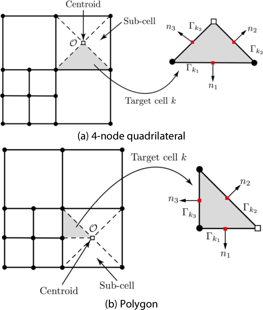
In this section, the basic idea behind the gradient smoothing approach within the framework of the FEM is briefly revisited. Liu et al. (2007a) introduced the gradient smoothing approach in the framework of the FEM, often called S-FEM, to improve linear triangular and bilinear quadrilateral elements. One of the remarkable aspects of S-FEM is the sub-division of finite elements, so-called sub-cells. Then, sub-cells are reconstructed to smoothing domains by different schemes where gradients are smoothed over the smoothing domains. Thus, strains are continuous over the smoothing domains but are discontinuous across the boundaries of smoothing domains, not elements (Liu and Nguyen, 2016). In the framework of S-FEM, not only triangular or quadrilateral cells but also arbitrary polygons can be used (Dai et al., 2007). This feature leads to quadtree meshes that can be employed in S-FEM without any further numerical treatments. Fig. 1 illustrates the cell-based S-FEM (CS-FEM) scheme that how to construct the smoothing domains for quadtree meshes. In general, for CS-FEM, the shape of a sub-cell follows the shape of the parent cell, such as a quadrilateral element cell is divided into four quadrilateral sub-cells and triangular element cell has three triangular sub-cells. However, since this work utilizes quadtree meshes, the 4-node quadrilateral element is divided into four triangular sub-cells as shown in Fig. 2(a). In quadtree mesh refinement, 5-node to 8-node polygons are possibly generated; therefore, the number of triangular sub-cells depends on the number of vertices of the parent element cell. For example, as shown in Fig. 2(b), a 5-node polygonal element cell is divided into 5 triangular sub-cells. As shown in Fig. 2, in the cell-based smoothed approximation, each sub-cell plays a role as the smoothing domain, where gradients are smoothed.

https://cdn.apub.kr/journalsite/sites/jcoseik/2023-036-05/N0040360502/images/Figure_jcoseik_36_05_02_F2.jpg

Fig. 2.

The cell-based smoothing scheme: (a) smoothing domain in quadrilateral cell and (b) smoothing domain in polygonal cell

In S-FEM approximation, the following infinitesimal strain $ε^{h}$ over the smoothing domain $Ω_{k}$ is considered:

(11)

ε^{h} (x_{k}) = \int_{Ω_{k}} ε^{h} (x) Φ (x) d Ω, \forall x \in Ω_{k}

where a point $x_{k}$ is located on the boundaries of the smoothing domain and the weight function 𝛷, along with its property, is given in Eqs. (12a) and (12b), respectively:

(12a)

\int_{Ω_{k}} Φ (x) d Ω = 1, Φ > 0

(12b)

Φ (x) = \{\begin{cases} \begin{matrix} 1 / A_{k} & x \in Ω_{k} \end{matrix} \\ \begin{matrix} 0 & x \notin Ω_{k} \end{matrix} \end{cases}

Therefore, Eq. (11) can be rewritten by means of the divergence theorem as follows:

(13)

\tilde{ɛ} (x_{k}) = \frac{1}{A_{k}} \int_{Ω_{k}}^{} ɛ (x) Φ (x) d Ω = \frac{1}{A_{k}} \int_{Γ_{k}}^{} n (x) u^{h} (x) d Ω

where $A_{k}$ is the area of the smoothing domain and $n (x)$ is the outward normal vector given at Gauss points located on the middle point of boundaries of the smoothing domain as shown in Fig. 2. In terms of the nodal displacements, Eq. (13) is rewritten as Eq. (14) as follows:

(14)

\tilde{ɛ} (x) = \sum_{I \in G_{k}} {\tilde{B}}_{I} (x) {u_{I}}^{h}

where $G_{k}$ is a set of nodes. The smoothed strain-displacement matrix for 2D is given in the following Eq. (15):

(15)

{\tilde{B}}_{I i} = [\begin{matrix} {\tilde{B}}_{I x} & 0 \\ 0 & {\tilde{B}}_{I y} \\ {\tilde{B}}_{I y} & {\tilde{B}}_{I x} \end{matrix}]

where

(16)

{\tilde{B}}_{I i} = \frac{1}{A_{k}} \int_{Γ_{k}} N_{I} (x) n_{i} (x) d Γ

where $N_{I}$ is the shape functions and $Γ_{k}$ is the boundaries of the smoothing domain. As shown in Fig. 2 and Eq. (16), the proposed S-FEM does not require an explicit form of shape functions. In other words, there is no isoparametric mapping. In addition, the interior Gauss integration is altered to line integration with one Gauss point at the middle of boundaries of the smoothing domain (please refer to Fig. 2). These salient features of S-FEM bring marked benefits that it can avoid over-estimation of the stiffness and is immune to highly distorted meshes.

Eq. (17) presents the discrete system equation for S-FEM:

(17)

\tilde{K} u = f \tilde{K} = \int_{Ω} {\tilde{B}}^{T} (x) C \tilde{B} (x) d Ω = \sum_{k = 1}^{n_{c}} \int_{Ω_{k}} {\tilde{B}}^{T} (x) C \tilde{B} (x) d Ω = \sum_{k = 1}^{n_{c}} {\tilde{B}}^{T} (x) C \tilde{B} (x) A_{k}

where $n_{c}$ is the number of target cells. The external force vector $f$ is obtained in the same manner in finite element approximation.

3.1 Quadtree refinement

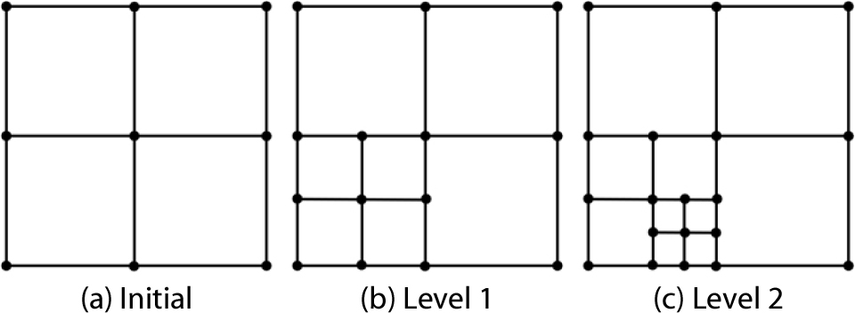
The quadtree mesh refinement is involved in this work for spatial discretization. As shown in Fig. 3, a quadrilateral mesh is sub-dividing into four cells with equal dimensions recursively. In general, this process lies in certain conditions, for instance, the solutions are concentrated or the geometric discontinuity exists. In this work, quadtree decomposition is facilitated along the crack surface. For interested readers, the details of the use of quadtree refinement can be referred to Natarajan et al. (2013) and references therein.

https://cdn.apub.kr/journalsite/sites/jcoseik/2023-036-05/N0040360502/images/Figure_jcoseik_36_05_02_F3.jpg

Fig. 3.

Quadtree decomposition in quadrilateral elements

3.2 Wachspress basis functions

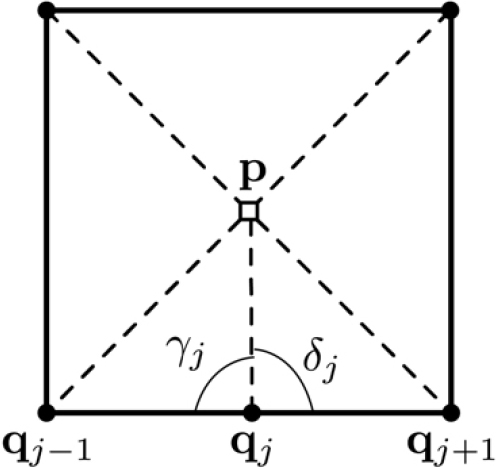
For $n$ -sided polygons, Wachspress (1971) introduced the rational basis functions to obtain nodal interpolation and linearity on the boundaries. Later, Warren et al. (2007) proposed the generalized Wachspress basis functions for simplex polygons and Meyer et al. (2002) suggested a simple form of a barycentric Wachspress basis function. We use the following simple form of Wachspress basis functions given in Eq. (18) in the smoothed FEM framework:

(18)

N_{j} (x) = \frac{w_{j} (x)}{\sum_{k} w_{k} (x)}

where w_j(x) is defined in the following Eq. (19):

(19)

w_{j} (x) = \frac{A (q_{j - 1}, q_{j}, q_{j + 1})}{A (q_{j - 1}, q_{j}, p) A (q_{j}, q_{j + 1}, p)} = \frac{\sin (γ_{j} + δ_{i j})}{\sin (γ_{j}) \sin (δ_{j}) ∥ p - q_{j} ∥^{2}} = \frac{\cot (γ_{j}) + \cot (δ_{j})}{∥ p - q_{j} ∥^{2}}

where the signed area of triangle $(p, q, r)$ is $A (p, q, r)$ and adjacent angles are $γ_{j}$ and $δ_{j}$ as given in Fig. 4.

https://cdn.apub.kr/journalsite/sites/jcoseik/2023-036-05/N0040360502/images/Figure_jcoseik_36_05_02_F4.jpg

Fig. 4.

Barycentric coordinates for an n-sided element

4. Numerical Tests

In this section, numerical results concerning the proposed adaptive quadtree S-FEM implementation into the framework of the phase-field method are investigated. The first example validates CS-FEM with a 4-node quadrilateral (Q4) element comparing FEM and CS-FEM with a 3-node triangular (T3) element. Then, a patch test for the implementation of the phase- field method is investigated in Section 4.2. In the following section, fracture problems are considered to evaluate the current approaches under different characteristics of cracks. Note that plane strain condition is considered for all tests.

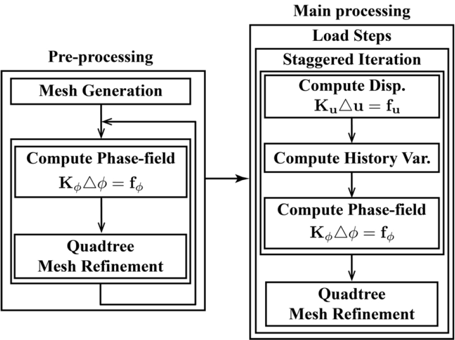
Fig. 5 illustrates a schematic flowchart of the pseudo-code of the proposed framework. In the pre-processing stage, an initial finite element mesh is discretized and the phase-field is computed to generate quadtree meshes. Next, the staggered iteration is employed in the main stage to compute displacements, history variables and the phase-field. Then, quadtree meshes are adaptively generated checking the threshold of the phase-field. The staggered iteration is repeated with increased load steps using refined quadtree meshes. For conducting the subsequent numerical tests, the proposed framework has been implemented in MATLAB 2019b, which runs on an AMD Ryzen 5 5600G processor clocked at 3.90GHz and is equipped with 32GB of RAM.

https://cdn.apub.kr/journalsite/sites/jcoseik/2023-036-05/N0040360502/images/Figure_jcoseik_36_05_02_F5.jpg

Fig. 5.

Main steps involved in the implementation of the propose framework

4.1 Cantilever beam

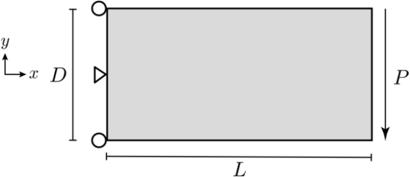
This section tests a cantilever beam as the validation for the proposed smoothed FEM. Fig. 6 depicts the geometry of the beam and boundary conditions. The length and height of the beam are $L \in \{0, 5\}$ m and $D \in \{- 1, 1\}$ m, respectively. The boundary conditions are imposed on the left end of the beam and the load $P$ =1N carries on the right side of the beam. Young’s modulus and Poisson’s ratio are $E$ =1000N/mm² and 𝜐=0.3.

https://cdn.apub.kr/journalsite/sites/jcoseik/2023-036-05/N0040360502/images/Figure_jcoseik_36_05_02_F6.jpg

Fig. 6.

Geometry and boundary conditions of a cantilever beam

The exact displacements and stresses can be found in Augarde and Deeks (2008):

$σ_{x x} = \frac{P (L - x) y}{I}, σ_{y y} = 0, τ_{x y} = - \frac{P}{2 I} (\frac{D^{2}}{4} - y^{2})$

$u_{x} = - \frac{P}{6 E I} [(6 L - 3 x) x + (2 + υ) (y^{2} - \frac{D^{2}}{4})]$

$u_{y} = - \frac{P}{6 E I} [3 υ y^{2} (L - x) + (4 + 5 υ) \frac{D^{2} x}{4} + (3 L - x) x^{2}]$

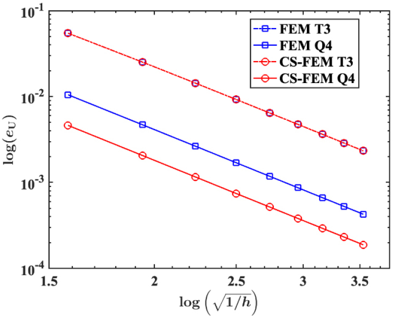
For this test, the following 9 levels of refined Q4 elements are used: 306, 650, 1,122, 1,722, 2,450, 3,306, 4,290, 5,402 and 6,642DOFs. Fig. 7 shows the convergence of the relative errors in displacements for FEM with Q4 and T3 elements and CS-FEM Q4 and T3 elements. As expected, Q4-CS-FEM yields more accurate results than Q4- and T3-FEMs, while T3-CS-FEM provides almost identical accuracy to T3-FEM.

https://cdn.apub.kr/journalsite/sites/jcoseik/2023-036-05/N0040360502/images/Figure_jcoseik_36_05_02_F7.jpg

Fig. 7.

Cantilever beam: convergence of the relative errors in displacements for FEM and S-FEM

4.2 Patch test

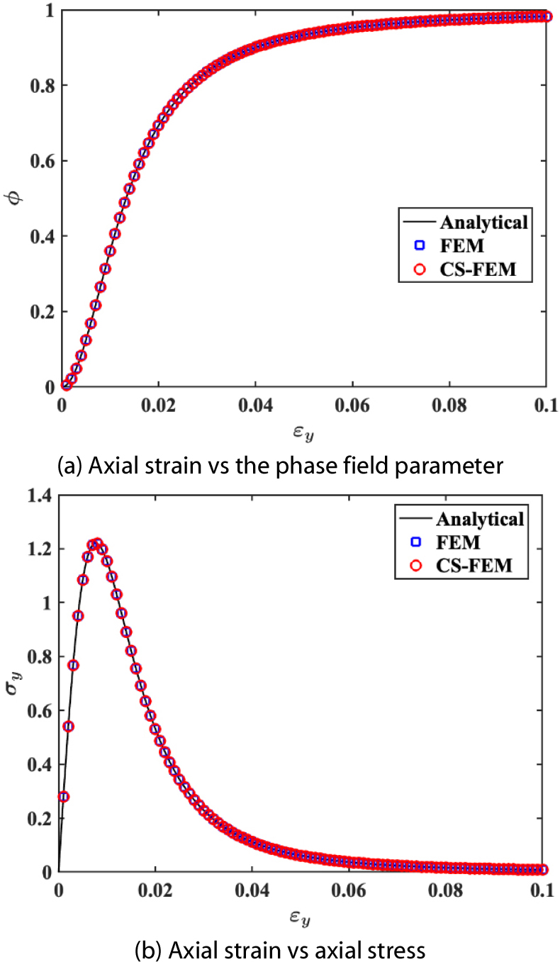
Next, a simple test of S-FEM implementation into the phase- field method with the analytical solution is examined. A unit square plate, viz. $L$ =1mm, under un-axial tension is used as shown in Fig. 8. The following material and the phase-field properties are chosen: Young’s modulus $E$ =210kN/mm², Poisson’s ratio 𝜐=0.3, critical energy release rate $G_{c}$ =5 × 10^-3kN/mm and the internal length scale $l_{0}$ =0.1mm. The displacement $\bar{u} =$ 0.1mm is applied on the top edge of the plate with $∆ \bar{u} =$ 1 × 10^-3mm increment. The analytical solutions, given by Molnár and Gravouil (2017), for this test can be found in Eq. (20):

(20a)

σ_{y, 0} = \frac{E (1 - υ)}{(1 + υ) (1 - 2 υ)} ε_{y}

(20b)

Ψ = \frac{1}{2} \frac{E (1 - υ)}{(1 + υ) (1 - 2 υ)} ε_{y}^{2}

(20c)

ϕ = \frac{2 Ψ}{\frac{G_{c}}{l_{0}} + 2 Ψ} = \frac{\frac{E (1 - υ)}{(1 + υ) (1 - 2 υ)} ε_{y}^{2}}{\frac{G_{c}}{l_{0}} + \frac{E (1 - υ)}{(1 + υ) (1 - 2 υ)} ε_{y}^{2}}

(20d)

σ_{y} = σ_{y, 0} (1 - ϕ)^{2}

where $ε_{y}$ is the axial strain and $σ_{y}$ is the axial stress under the damaged condition.

https://cdn.apub.kr/journalsite/sites/jcoseik/2023-036-05/N0040360502/images/Figure_jcoseik_36_05_02_F8.jpg

Fig. 8.

Geometry and boundary conditions of patch test: uni-axial tension

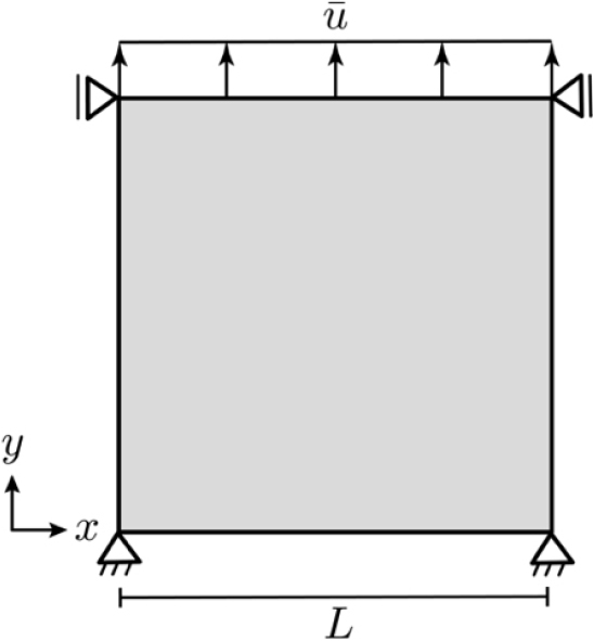
Fig. 9 illustrates the evolution of the phase-field parameter and the axial stress as a function of the axial strain. As shown in Fig. 9(a), the evolution of the phase-field parameter is zero (undamaged) to one (fully damaged). As the phase-field parameter evolves, there is a noticeable decline in the load-bearing capacity of the material stiffness as shown in Fig. 9(b). These results show that the current approach meets an excellent agreement with the analytical solutions.

https://cdn.apub.kr/journalsite/sites/jcoseik/2023-036-05/N0040360502/images/Figure_jcoseik_36_05_02_F9.jpg

Fig. 9.

Patch tests: comparison of the phase-field parameter as a function of the axial strain and the axial stress as a function of the axial strain

4.3 Plate with the crack

Next, we consider the two-dimensional domains with straight single and double cracks undergoing tension and shear. For the following test, a unit square plate with Lame’s first parameter 𝜆=121.15kN/mm² and the shear modulus 𝜇=80.77kN/mm², equivalent to $E$ =2.1 × 10⁵kN/mm² and 𝜈=0.3, is evaluated. The critical energy release rate $G_{c}$ =2.7 × 10kN/mm and the internal length scale $l_{0}$ =0.011mm are also considered.

4.3.1 Single crack with tension

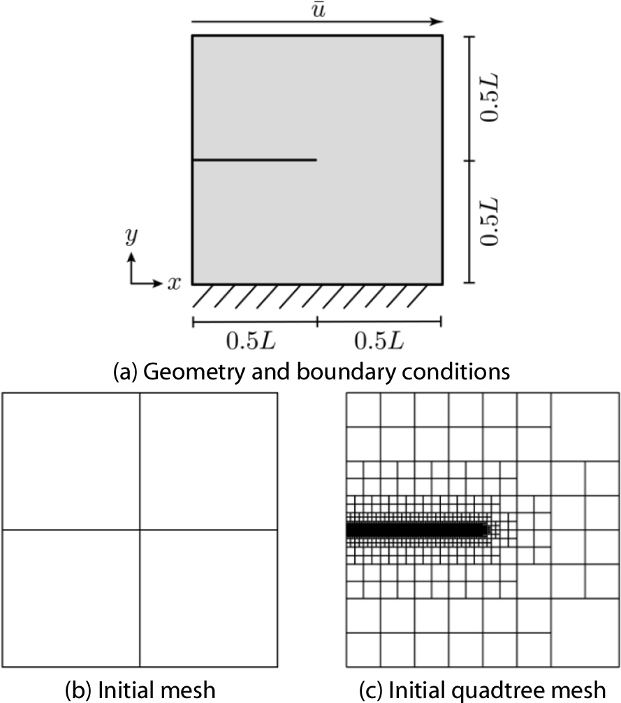
First, the plate with a straight crack with tension is investigated. The crack is located at $x \in$ {0,0.5}mm and $y$ =0.5mm as shown in Fig. 10(a). Displacement $\bar{u}$ is imposed on the top edge of the plate with $∆ \bar{u} =$ 1.99 × 10^-4mm up to $\bar{u}$ 4.78 × 10^-3mm and then $∆ \bar{u} =$ 1.5 × 10^-6mm up to $\bar{u}$ 6 × 10^-3mm which to reach the failure.

https://cdn.apub.kr/journalsite/sites/jcoseik/2023-036-05/N0040360502/images/Figure_jcoseik_36_05_02_F10.jpg

Fig. 10.

Plate with a single crack with tension: (a) geometry and boundary conditions, (b) initial finite element mesh and (c) refined initial quadtree mesh (11,416DOFs)

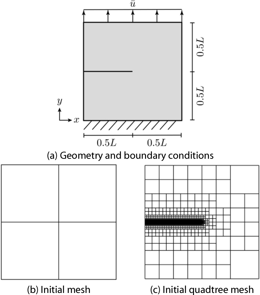
In the beginning, the plate is discretized into 2 × 2 elements and then quadtree meshes are refined along the crack surface as shown in Figs. 10(b) and 10(c). Then meshes are adaptively refined along the path of the crack growth up to the failure of the specimen. Fig. 11 illustrates quadtree meshes and the phase-field parameters of FEM and CS-FEM. The force-displacement curve of CS-FEM is given in Fig. 12 comparing FEM and the reference solution (Miehe et al., 2010b). It can be observed that the proposed approach shows relatively comparable failure patterns like FEM.

https://cdn.apub.kr/journalsite/sites/jcoseik/2023-036-05/N0040360502/images/Figure_jcoseik_36_05_02_F11.jpg

Fig. 11.

Plate with a single crack with tension: adaptively refined quadtree meshes and the phase-field parameter ( $\bar{u}$ 0.6 × 10^-3mm)

https://cdn.apub.kr/journalsite/sites/jcoseik/2023-036-05/N0040360502/images/Figure_jcoseik_36_05_02_F12.jpg

Fig. 12.

Plate with a single crack with tension: load-displacement curve

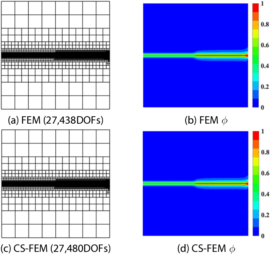
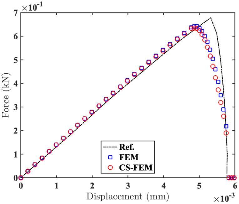
Table 1 presents the simulation time for the single crack with the tension problem. Unlike edge-based and node-based S-FEM, where the bandwidth of their stiffness matrix is wider than FEM, the bandwidth of the proposed CS-FEM is the same as that of FEM. Hence, in general problems, the computational times of CS-FEM and the standard FEM are similar. However, in the context of adaptive quadtree mesh refinement, FEM elements with hanging nodes require more integration points compared to the proposed CS-FEM, where the integration points remain constant. This numerical aspect, as given in Table 1, results in the proposed CS-FEM requiring relatively more degrees of freedom but remarkably shorter simulation time than FEM in the present study.

Table 1.

Comparison of the numerical result of single crack with tension: FEM and CS-FEM

	FEM	CS-FEM
Num. of load steps	838	838
Num. of nodes	13,719	13,740
Num. of elements	12,892	12,913
Computational time	54.82 (mins.)	38.82 (mins.)

4.3.2 Single crack with shear

The next test is the plate with a straight crack with shear. The geometry and boundary conditions of the problem are given in Fig. 13(a). The crack is in the same position as the previous test in Section 4.3.1. Displacement is increased with $∆ \bar{u} =$ 8.8 × 10^-4mm up to $\bar{u}$ 8 × 10^-3mm and then $∆ \bar{u} =$ 2.45 × 10^-4mm is applied until when $\bar{u}$ 2 × 10^-2mm.

https://cdn.apub.kr/journalsite/sites/jcoseik/2023-036-05/N0040360502/images/Figure_jcoseik_36_05_02_F13.jpg

Fig. 13.

Plate with a single crack with tension: (a) geometry and boundary conditions, (b) initial finite element mesh and (c) refined initial quadtree mesh (11,416DOFs)

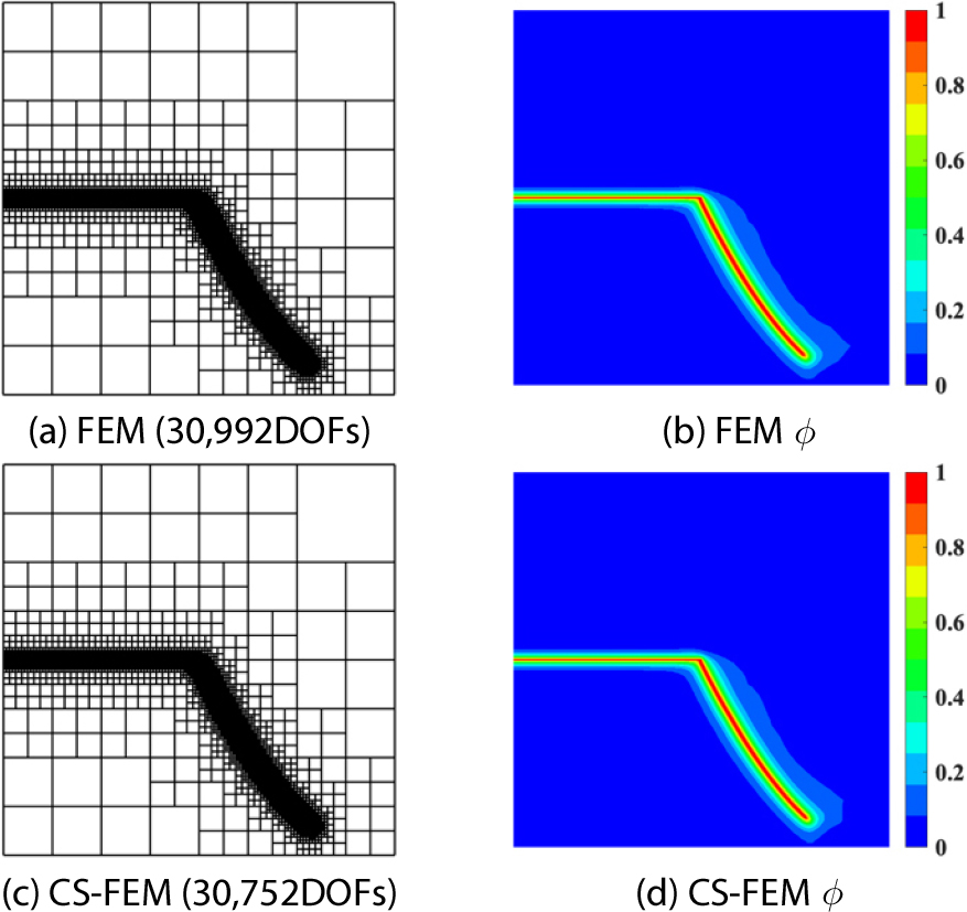
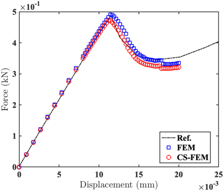
Figs. 14(a) and 14(c) show the adaptive quadtree decomposition and the crack propagation path can be found in Figs. 14(b) and 14(d). Fig. 15 depicts the curve of the relationship between displacement and load. Compared to FEM, the present approach yields good agreement with the reference solution (Miehe et al., 2010b).

https://cdn.apub.kr/journalsite/sites/jcoseik/2023-036-05/N0040360502/images/Figure_jcoseik_36_05_02_F14.jpg

Fig. 14.

Plate with a single crack with shear: adaptively refined quadtree meshes and the phase-field parameter ( $\bar{u}$ 2 × 10^-2mm)

https://cdn.apub.kr/journalsite/sites/jcoseik/2023-036-05/N0040360502/images/Figure_jcoseik_36_05_02_F15.jpg

Fig. 15.

Plate with a single crack with shear: load-displacement curve

Results, numbers of nodes and elements of quadtree meshes and simulation time, of the single crack with the shear problem are given in Table 2. In contrast to the single crack with the tension problem, CS-FEM has the need for comparatively fewer nodes and elements. Additionally, the computational cost of the proposed approach is reasonably cheaper than FEM.

Table 2.

Comparison of the numerical result of single crack with shear: FEM and CS-FEM

	FEM	CS-FEM
Num. of load steps	59	59
Num. of nodes	15,496	15,473
Num. of elements	14,563	14,536
Computational time	14.03 (mins.)	11.05 (mins.)

4.3.3 Double cracks with tension

The numerical experiment ends with asymmetric cracks at both ends of the plate with tension in this section. The geometry and boundary conditions are given in Fig. 16(a) with the initial crack length $D$ \0.4mm and $h$ =0.1mm. The domain is discretized into 10 × 10 elements at first and quadtree meshes are generated with 9,230DOFs along both crack surfaces (see Figs. 16(b) and 16(c)).

https://cdn.apub.kr/journalsite/sites/jcoseik/2023-036-05/N0040360502/images/Figure_jcoseik_36_05_02_F16.jpg

Fig. 16.

Plate with double cracks with tension: (a) geometry and boundary conditions, (b) initial finite element mesh and (c) refined initial quadtree mesh (11,416DOFs)

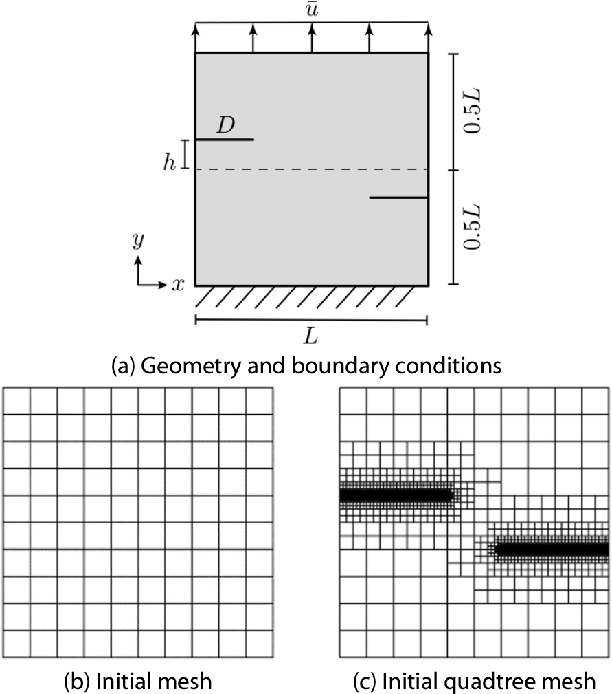
The tension is applied with: $∆ \bar{u} =$ 4.78 × 10^-3mm for 25steps, then it reduced to $∆ \bar{u} =$ 1.5 × 10^-6mm for the rest simulation, which to reach $\bar{u}$ 7.5 × 10^-3mm.

Fig. 17 shows refined quadtree meshes and the crack propagation path for the test. For FEM, quadtree refinement generates 13,900DOFs along the crack path while 13,874DOFs are decomposed in CS-FEM. The proposed CS-FEM provides the expected crack propagation path when double cracks are involved.

https://cdn.apub.kr/journalsite/sites/jcoseik/2023-036-05/N0040360502/images/Figure_jcoseik_36_05_02_F17.jpg

Fig. 17.

Plate with double cracks with tension: adaptively refined quadtree meshes and the phase-field parameter ( $\bar{u}$ 7.5 × 10^-3mm)

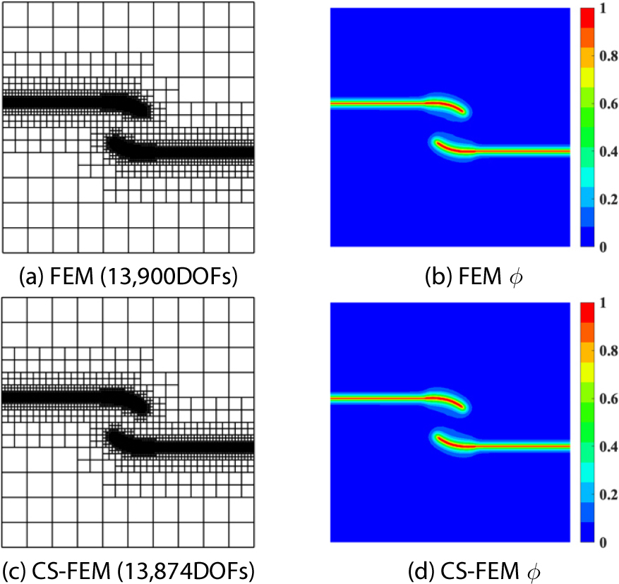
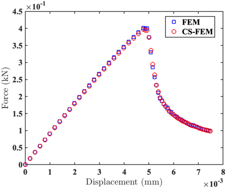
Fig. 18 illustrates the reaction force as a function of the applied displacements, showing energy degradation.

Lastly, the comparison of computational time with respect to the adaptive quadtree elements and nodes for the proposed approach and FEM is given in Table 3. The proposed CS-FEM requires relatively fewer DOFs than FEM, but its simulation time is approximately half that of FEM. Consequently, the present method needs marginally fewer or more DOFs; however, it yields cheaper computational costs retaining the comparable accuracy to FEM.

https://cdn.apub.kr/journalsite/sites/jcoseik/2023-036-05/N0040360502/images/Figure_jcoseik_36_05_02_F18.jpg

Fig. 18.

Plate with double cracks with tension: load-displacement curve

Table 3.

Comparison of the numerical result of double cracks with tension: FEM and CS-FEM

	FEM	CS-FEM
Num. of load steps	1,838	1,838
Num. of nodes	6,950	6,937
Num. of elements	6,247	6,232
Computational time	74.76 (mins.)	44.57 (mins.)

5. Conclusion

In this work, a staggered phase-field method is implemented into the framework of smoothed finite element method. To avoid the finer mesh generation burden and to achieve computational efficiency, an adaptive quadtree mesh decomposition scheme is incorporated into S-FEM.

In the method, the elastic displacements and the phase-field parameters are decoupled and solved separately. To link both processes, the historical variables of the potential energy are employed.

The crack propagation is represented by the phase-field parameters as zero (no damage) and one for completely damaged.

The proposed S-FEM implementation is validated with the result available in the literature. The results show that the adaptive S-FEM of the phase-field method produces a good agreement with the reference solution, requiring fewer DOFs less computational effort than regular meshes at a similar level of accuracy.

Acknowledgements

This research is supported by the Basic Science Research Program through the National Research Foundation of Korea (NRF) funded by the Ministry of Education (2016R1A6A1 A03012812).

References

Ambati, M., Gerasimov, T., De Lorenzis, L. (2014) A Review on Phase-Field Models of Brittle Fracture and a New Fast Hybrid Formulation, Comput. Mech., 55, pp.383~405. 10.1007/s00466-014-1109-y

Amor, H., Marigo, J.-J., Maurini, C. (2009) Regularized Formulation of the Variational Brittle Fracture with Unilateral Contact: Numerical Experiments, J. Mech. & Phys. Solids, 57, pp. 1209~1229. 10.1016/j.jmps.2009.04.011

Augarde, C.E., Deeks, A.J. (2008) The Use of Timoshenko's Exact Solution for a Cantilever Beam in Adaptive Analysis, Finite Elem. Anal. & Des., 44, pp.595~601. 10.1016/j.finel.2008.01.010

Bordas, S.P.A., Rabczuk, T., Nguyen-Xuan, H., Nguyen, V.P., Natarajan, S., Bog, T., Quan, D.M., Hiep, N.V. (2010) Strain Smoothing in FEM and XFEM, Comput. & Struct., 88, pp.1419~1443. 10.1016/j.compstruc.2008.07.006

Bourdin, B., Francfort, G.A., Marigo, J.-J. (2000) Numerical Experiments in Revisited Brittle Fracture, J. Mech. & Phys. Solids, 48, pp.797~826. 10.1016/S0022-5096(99)00028-9

Dai, K.Y., Liu, G.R., Nguyen, T.T. (2007) An -sided Polygonal Smoothed Finite Element Method (SFEM) for Solid Mechanics, Finite Elem. Anal. & Des., 43, pp.847~860. 10.1016/j.finel.2007.05.009

Finkel, R.A., Bentley, J.L. (1974) Quad Trees a Data Structure for Retrieval on Composite Keys, Acta Inform., 4, pp.1~9. 10.1007/BF00288933

Francfort, G.A., Marigo, J.-J. (1998) Revisiting Brittle Fracture as an Energy Minimization Problem, J. Mech. & Phys. Solids, 46, pp.1319~1342. 10.1016/S0022-5096(98)00034-9

Fries, T.-P., Belytschko, T. (2010) The Extended/Generalized Finite Element Method: An Overview of the Method and Its Applications, Int. J. Numer. Methods Eng., 84, pp.253~304. 10.1002/nme.2914

Griffith, A.A. (1921) The Phenomenon of Rupture and Flow in Solids, Philos. Trans. Royal Soc. Lond., Series A, Containing Papers of a Mathematical or Physical Character, 221, pp. 163~198. 10.1098/rsta.1921.0006

Hirshikesh, Natarajan, S., Annabattula, R.K. (2018) A FEniCS Implementation of the Phase Field Method for Quasi-static Brittle Fracture, Front. Struct. & Civil Eng., 13, pp.380~396. 10.1007/s11709-018-0471-9

Lee, C.K., Singh, I.V., Natarajan, S. (2022) A Cell-based Smoothed Finite Element Method for Gradient Elasticity, Eng. with Comput., 39, pp.925~942. 10.1007/s00366-022-01734-2

Liu, G.R., Dai, K.Y., Nguyen, T.T. (2007a) A Smoothed Finite Element Method for Mechanics Problems, Comput. Mech., 39, pp.859~877. 10.1007/s00466-006-0075-4

Liu, G.R., Nguyen, T.T. (2016) Smoothed Finite Element Methods, CRC Press, Boca Raton. 10.1201/EBK1439820278

Liu, G.R., Nguyen, T.T., Dai, K.Y., Lam, K.Y. (2007b) Theoretical Aspects of the Smoothed Finite Element Method (SFEM), Int. J. Numer. Methods Eng., 71, pp.902~930. 10.1002/nme.1968

Meyer, M., Lee, H., Barr, A., Desbrun, M. (2002) Generalized Barycentric Coordinates for Irregular Polygons, J. Graph. Tools, 7, pp.13~22. 10.1080/10867651.2002.10487551

Miehe, C., Hofacker, M., Welschinger, F. (2010a) A Phase Field Model for Rate-independent Crack Propagation: Robust Algorithmic Implementation based on Operator Splits, Comput. Methods Appl. Mech. & Eng., 199, pp.2756~2778. 10.1016/j.cma.2010.04.011

Miehe, C., Welschinger, F., Hofacker, M. (2010b) Thermodynamically Consistent Phase-field Models of Fracture: Variational Principles and Multi-field FE Implementation, Int. J. Numer. Methods Eng., 83, pp.1273~1311. 10.1002/nme.2861

Moës, N., Belytschko, T. (2002) Extended Finite Element Method for Cohesive Crack Growth, Eng. Fract. Mech., 69, pp.813~ 833. 10.1016/S0013-7944(01)00128-X

Molnár, G., Gravouil, A. (2017) 2D and 3D Abaqus Implementation of a Robust Staggered Phase-field Solution for Modeling Brittle Fracture, Finite Elem. Anal. & Des., 130, pp.27~38. 10.1016/j.finel.2017.03.002

Natarajan, S., Ooi, E.T., Song, C. (2013) Finite Element Computations on Quadtree Meshes: Strain Smoothing and Semi-analytical Formulation, Math.: Numer. Anal., arXiv, 1310.2913.

Surendran, M., Natarajan, S., Bordas, S.P.A., Palani, G.S. (2017) Linear Smoothed Extended Finite Element Method, Int. J. Numer. Methods Eng., 112, pp.1733~1749. 10.1002/nme.5579

Wachspress, E.L. (1971) A Rational Basis for Function Approximation, IMA J. Appl. Math., 8, pp.57~68. 10.1093/imamat/8.1.57

Warren, J., Schaefer, S., Hirani, A., Desbrun, A. (2007) Barycentric Coordinates for Convex Sets, Adv. Comput. Mech., 3, pp. 319~338. 10.1007/s10444-005-9008-6

Yoo, H.-S., Kim, H.-S. (2016) Simulation of Multi-Cracking in a Reinforced Concrete Beam by Extended Finite Element Method, J. Comput. Struct. Eng. Inst. Korea, 29, pp.201~208. 10.7734/COSEIK.2016.29.2.201

Zeng, W., Liu, G.R. (2018) Smoothed Finite Element Methods (S-FEM): An Overview and Recent Development, Arch. Comput. Methods Eng., 25, pp.397~435. 10.1007/s11831-016-9202-3

Zhuang, X., Zhou, S., Huynh, G.D., Areias, P., Rabczuk, T. (2022) Phase Field Modeling and Computer Implementation: A Review, Eng. Fract. Mech., 262, p.108234. 10.1016/j.engfracmech.2022.108234

Journal of the Computational Structural Engineering Institute of Korea ISSN:1229-3059(Print) 2287-2302(Online) 한국전산구조공학회 논문집

Preview

Quasi-brittle and Brittle Fracture Simulation Using Phase-field Method based on Cell-based Smoothed Finite Element Method

ABSTRACT

MAIN

(1)

(2)

Fig. 1.

Solid body with crack topology

(3)

(4)

(5a)

(5b)

(6a)

(6b)

(7)

(8)

(9a)

(9b)

(10a)

(10b)

(10c)

(10d)

Fig. 2.

The cell-based smoothing scheme: (a) smoothing domain in quadrilateral cell and (b) smoothing domain in polygonal cell

(11)

(12a)

(12b)

(13)

(14)

(15)

(16)

(17)

Fig. 3.

Quadtree decomposition in quadrilateral elements

(18)

(19)

Fig. 4.

Barycentric coordinates for an n-sided element

Fig. 5.

Main steps involved in the implementation of the propose framework

Fig. 6.

Geometry and boundary conditions of a cantilever beam

Fig. 7.

Cantilever beam: convergence of the relative errors in displacements for FEM and S-FEM

(20a)

(20b)

(20c)

(20d)

Fig. 8.

Geometry and boundary conditions of patch test: uni-axial tension

Fig. 9.

Patch tests: comparison of the phase-field parameter as a function of the axial strain and the axial stress as a function of the axial strain

Fig. 10.

Plate with a single crack with tension: (a) geometry and boundary conditions, (b) initial finite element mesh and (c) refined initial quadtree mesh (11,416DOFs)

Fig. 11.

Plate with a single crack with tension: adaptively refined quadtree meshes and the phase-field parameter (u¯0.6 × 10-3mm)

Fig. 12.

Plate with a single crack with tension: load-displacement curve

Table 1.

Comparison of the numerical result of single crack with tension: FEM and CS-FEM

Fig. 13.

Plate with a single crack with tension: (a) geometry and boundary conditions, (b) initial finite element mesh and (c) refined initial quadtree mesh (11,416DOFs)

Fig. 14.

Plate with a single crack with shear: adaptively refined quadtree meshes and the phase-field parameter (u¯2 × 10-2mm)

Fig. 15.

Plate with a single crack with shear: load-displacement curve

Table 2.

Comparison of the numerical result of single crack with shear: FEM and CS-FEM

Fig. 16.

Plate with double cracks with tension: (a) geometry and boundary conditions, (b) initial finite element mesh and (c) refined initial quadtree mesh (11,416DOFs)

Fig. 17.

Plate with double cracks with tension: adaptively refined quadtree meshes and the phase-field parameter (u¯7.5 × 10-3mm)

Fig. 18.

Plate with double cracks with tension: load-displacement curve

Table 3.

Comparison of the numerical result of double cracks with tension: FEM and CS-FEM

Acknowledgements

References

Plate with a single crack with tension: adaptively refined quadtree meshes and the phase-field parameter ( $\bar{u}$ 0.6 × 10^-3mm)

Plate with a single crack with shear: adaptively refined quadtree meshes and the phase-field parameter ( $\bar{u}$ 2 × 10^-2mm)

Plate with double cracks with tension: adaptively refined quadtree meshes and the phase-field parameter ( $\bar{u}$ 7.5 × 10^-3mm)