Comparison among Methods of Modeling Epistemic Uncertainty in Reliability Estimation

Yoo Min Young; Kim Nam Ho; Choi Joo Ho

doi:10.7734/COSEIK.2014.27.6.605

Preview

Journal of the Computational Structural Engineering Institute of Korea. 2014. 605-613
https://doi.org/10.7734/COSEIK.2014.27.6.605

Comparison among Methods of Modeling Epistemic Uncertainty in Reliability Estimation

신뢰성 해석을 위한 인식론적 불확실성 모델링 방법 비교

Yoo Min Young

Kim Nam Ho

Choi Joo Ho^†^*

School of Aerospace and Mechanical Engineering, Korea Aerospace University, Goyang, 412-791, Korea

Department of Mechanical and Aerospace Engineering, University of Florida, Gainesville, Florida, 32611, USA

Department of Aerospace and Mechanical Engineering, Korea Aerospace University, Goyang, 412-791, Korea

•^*Corresponding author Choi, Joo Ho jhchoi@kau.ac.kr

License (open-access, http://creativecommons.org/licenses/by-nc/3.0/):

This is an Open-Access article distributed under the terms of the Creative Commons Attribution Non-Commercial License (http://creativecommons.org/licenses/by-nc/3.0) which permits unrestricted non-commercial use, distribution, and reproduction in any medium, provided the original work is properly cited.

ABSTRACT

Epistemic uncertainty, the lack of knowledge, is often more important than aleatory uncertainty, variability, in estimating reliability of a system. While the probability theory is widely used for modeling aleatory uncertainty, there is no dominant approach to model epistemic uncertainty. Different approaches have been developed to handle epistemic uncertainties using various theories, such as probability theory, fuzzy sets, evidence theory and possibility theory. However, since these methods are developed from different statistics theories, it is difficult to interpret the result from one method to the other. The goal of this paper is to compare different methods in handling epistemic uncertainty in the view point of calculating the probability of failure. In particular, four different methods are compared; the probability method, the combined distribution method, interval analysis method, and the evidence theory. Characteristics of individual methods are compared in the view point of reliability analysis.

신뢰성 해석을 수행할 때 정보부족으로 인해 발생하는 인식론적 불확실성(epistemic uncertainty)은 고유의 변동성에 의해 존재하는 내재적 불확실성(aleatory uncertainty)보다 더 중요하게 다뤄야 한다. 그러나 그동안 개발된 확률이론은 주로 내재적 불확실성을 모델링하는데 이용된 반면, 인식론적 불확실성의 모델링에 대해서는 아직 확실한 접근법이 없었다. 최근 이를 위해 probability theory를 포함한 여러 접근법들이 제시되고 있지만 이들은 서로 다른 통계적 이론들을 바탕으로 도출되었기 때문에, 각 방법들의 결과들을 이해하는데 어려움이 있었다. 본 연구에서는 고장 확률을 계산하는 문제를 가지고 이러한 방법들이 인식론적 불확실성을 어떻게 다루는지를 비교, 분석하였다. 이를 위해 probability method, combined distribution method, interval analysis method 그리고 evidence theory를 대상으로 신뢰도 분석문제에 대해 각 방법들의 특징들을 비교하였으며, 그 결과는 다음과 같다. 입력변수의 확률분포 형태를 알 수 있다면 probability method가 가장 우수하나, 이를 전혀 모르면 interval method를 사용해야 한다. 그러나 계산비용 면에서는 두 방법이 유사하므로 결국 입력변수의 확률특성 정보가 얼마나 있느냐에 따라 방법을 선택한다. Combined distribution method는 failure probability의 평균만 제공하므로 사용하지 않는 것이 좋다. 다만 이 방법은 계산비용이 매우 적게 드는 장점이 있다. Evidence theory는 probability와 interval 방법의 중간에 해당하며, 구간별 probability assignment를 세분화 할수록 probability결과에 접근한다. 이 방법은 계산비용이 가장 높은 것이 문제이다.

Keywords

epistemic uncertainty, reliability, interval method, evidence theory, probability method

인식론적 불확실성, 신뢰성, 간격법, 증거이론, 확률이론

MAIN

1. Introduction

In the reliability analysis of a system, epistemic uncertainty, which represents a lack of knowledge, is often more encountered than the aleatory uncertainty, which represents a natural variability of parameters. While there have been a widespread efforts to model the aleatory uncertainty throughout decades, there have been much less attention to the modeling of epistemic uncertainty. Recently, a couple of different approaches have been developed to handle the epistemic uncertainties as was mentioned in (Ferson et al., 2004) and (Kari et al.. 2011). These includes probability theory(Helton et al.. 1993), fuzzy sets or possibility theory(Zadeh, 1999), and evidence theory (Shafer, 1976; Dempster, 1967). However, since these methods are developed from different statistics theories, it is not easy to interpret the result from one method to the other. Therefore, this paper addresses the comparison of these methods for handling epistemic uncertainty in view of calculating the probability of failure.

It should be stressed out that we focus on describing characteristics of different approaches instead of suggesting a good approach. Here, we examine four approaches in modeling epistemic uncertainty: the probability method, the combined distribution method, the interval analysis method and the evidence theory. The first two methods, also known as second-order probability approach, model epistemic uncertainty with a distribution. The first method separates epistemic uncertainty from aleatory uncertainty and uses double- loop Monte Carlo simulation(MCS) to calculate the distribution of reliability. The second method, on the other hand, integrates epistemic uncertainty with aleatory uncertainty to predict combined distribution, whose results are equivalent to the mean of reliability from the first method. The interval analysis method is the simplest way to propagate epistemic uncertainty into interval of reliability. This method is a special case of the probability based method with separated epistemic uncertainty modeling. The epistemic uncertainty is defined with a bounded uniform distribution and the corresponding reliability bounds. Evidence theory models epistemic uncertainty with sets of intervals. A basic probability is assigned for each interval and intervals may overlap each other or have a gap.

We demonstrate these four approaches with a simple example of failure strength estimation. There is aleatory uncertainty in the failure strength due to inherent material variability. The source of epistemic uncertainty is from estimating the distribution of failure strength using a finite number of samples; i.e., statistical uncertainty. We will present how to interpret the epistemic uncertainty in the probability of failure for different approaches.

2. Aleatory and Epistemic Uncertainty

In the case of time-independent structural systems, it is often convenient to use a limit-state function in order to describe a reliability of a system. In this paper, the following form of limit-state function is used to determine the safety and failure of the system:

G = S - R

(1)

where, in the case of strength of material, S is the failure strength of a material, and R is the stress applied to the structure. The system is considered safe when G > 0 and failed with G ≤ 0. When the material strength or applied stress are uncertain, the safety of the system is evaluated in terms of reliability or, equivalently, the probability of failure defined as

P_{F} = P [G \leq 0]

(2)

where stands for the probability of the event in the bracket.

S_{true} ~ N (μ_{t r u e}, σ_{t r u e})

(3)

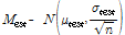
In order to simplify the discussion, it is assumed that there is no uncertainty in the applied stress; that is, the failure strength is the only source of uncertainty. Due to inherent variability of the material, it is assume that the failure strength is normally distributed; that is,

where μ_true and σ_true are, respectively, the mean and standard deviation of the true strength of the material, which are also called the distribution parameters. The uncertainty S_true is inherent variability and called aleatory uncertainty.

Unfortunately, the true distribution parameters of failure strength are unknown, and it can only be estimated through tests. When n number of specimens are used to estimate the failure strength, the estimated distribution of the failure strength becomes

S_{test} ~ N (μ_{t e s t}, σ_{t e s t})

(4)

where μ_test and σ_test are, respectively, the sample mean and standard deviation of test. Due to sampling error, the distribution parameters from test are different from the true ones. Of course, when infinite test samples are used, S_test will converge to S_true. However, since a finite number of samples are used, the estimated distribution parameters have epistemic uncertainty(i.e., sampling uncertainty or statistical uncertainty). From the classical probability theory, the uncertainty in the estimated mean and standard deviation can be expressed by

M_{est} ~ N (μ_{t e s t}, \frac{σ_{t r u e}}{\sqrt{n}})

(5)

https://cdn.apub.kr/journalsite/sites/jcoseik/2014-027-06/17TK122014270611/images/10.7734.27.6.605.F124.png

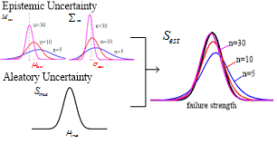
Figure 1

Illustration of the concept of aleatory and epistemic uncertainty of the failure strength distribution

\sum_{test} ~ \frac{σ_{t e s t}}{\sqrt{n - 1}} X (n - 1)

(6)

where X(n-1) is the chi-distribution of order n-1. Fig. 1 illustrates the concept of aleatory and epistemic uncertainty of the failure strength distribution

The source of epistemic uncertainty in Eqs. (5) and (6) are from sampling error. In general, however, different sources of epistemic uncertainty exist, such as modeling error, numerical error, etc. Although the statistical uncertainty in Eqs. (5) and (6) is given in the form of a distribution, epistemic uncertainty is not random by nature; that is, the true mean and standard deviation will be a single value, but their values are unknown. In this regard, the PDF of the distributions in Eqs. (5) and (6) should be interpreted as the shape of knowledge about the parameter. For example, Eq. (5) can be interpreted that the likelihood of μ_test being μ_true is higher than any other values.

When both aleatory and epistemic uncertainties exist, designer must determine a conservative failure strength in order to compensate for both uncertainties. For example, when there exists aleatory uncertainty only, designer can determine the 90 percentile of the distribution as a conservative failure strength. When epistemic uncertainty also exists, however, the 90 percentile cannot be determined as a single value, rather it becomes a distribution by itself. A designer must consider the effect of epistemic uncertainty when he or she chooses a conservative failure strength.

The conservative estimate of failure strength for both aleatory and epistemic uncertainty has already been implemented aircraft design. When coupon tests are used to estimate a conservative failure strength of an aluminum material, it is required to be estimated using A- or B-basis approach(U.S. Department of Defense, 2002). In the case of B-basis, for example, the conservative failure strength is estimated by 90 percentile with 95% confidence. The 90 percentile is for aleatory uncertainty, while 95% confidence is for epistemic uncertainty.

In the case when the epistemic uncertainty is represented by a probability distribution as in Eqs. (5) and (6), the probability theory can be used to calculate the effect of both aleatory and epistemic uncertainty, but it may not be straightforward if different methods of representing epistemic uncertainty are employed. In the following sections, four different methods of representing epistemic uncertainty are explained in the view point of conservative estimation of the failure strength: (1) the probability method, (2) the combined distribution method, (3) the interval analysis method and (4) the Dempster-Shafer evidence theory.

In order to make the discussions in the following section simple and consistent, we further simplify the epistemic uncertainty. It is assumed that epistemic uncertainty only exists in the estimated mean, M_est, not in the estimated standard deviation. In addition, it is further assumed that the epistemic uncertainty in the mean is uniformly distributed. This simplification is necessary because some methods do not use probability distribution to represent epistemic uncertainty. Table 1 shows the distribution parameters for both aleatory and epistemic uncertainty.

Table 1

Distribution parameters for aleatory and epistemic uncertainty



Failure strength
Estimated mean	(200,250)
True mean	225
Estimated standard deviation	20
Applied stress	R=190

3. Methods of Representing Epistemic Uncertainty

3.1 Probability method

The probability method is the most common approach in representing both epistemic and aleatory uncertainty. In this approach, the epistemic uncertainty is given in the form of a probability distribution. In the case of sampling error(i.e., statistical uncertainty), the epistemic uncertainties in the mean and standard deviation can be represented by normal and chi distributions, respectively, as shown in Eqs. (5) and (6). In the case of modeling error, since the epistemic uncertainty is related to the lack of knowledge, a uniform distribution is frequently used. However, it is important to note that even if the epistemic uncertainty is represented in the form of probability distribution, its interpretation should be different from that of aleatory uncertainty. That is, there is no randomness in epistemic uncertainty, but the probability distribution is used to shape the form of knowledge regarding the uncertain variable. Therefore this method is preferable when the information on the epistemic uncertainty is detail enough, such as the case of sampling error, so that the probability distribution of the epistemic uncertainty can be formed.

The problem formulation in Section 2 is based on the situation where the form of probability distribution for an uncertain variable is known, but the distribution parameters governing the distribution are uncertain. In such a case, the estimated failure strength essentially becomes a distribution of distributions. The estimated distribution of the failure strength can be obtained using a double-loop Monte Carlo simulation(MCS), as shown in Fig. 2.

https://cdn.apub.kr/journalsite/sites/jcoseik/2014-027-06/17TK122014270611/images/10.7734.27.6.605.F100.png

Figure 2

Double-loop Monte Carlo simulation for estimated distribution of failure strength

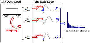
In the figure, the outer loop generates n samples from the estimated mean distribution, M_est~U(200,250), from which n sets of normal distributions, , can be defined. In the inner-loop, m samples of failure strengths are generated from each , which represents aleatory uncertainty. Since the failure strength is normally distributed, it is also possible that the inner-loop can be analytically calculated without generating samples.

For each given sample from epistemic uncertainty, the aleatory uncertainty is used to build a probability distribution, , from which the probability of failure, , can be calculated. By collecting all samples, a distribution of probability of failure can be obtained, which represents the epistemic uncertainty. A conservative estimate of the probability of failure, , can be obtained by taking the 90 percentile of the distribution. Therefore, the effect of aleatory uncertainty is considered by calculating , while that of epistemic uncertainty is considered by calculating .

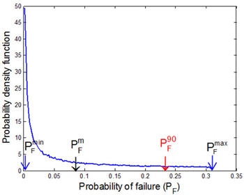
For the given example, the PDF of the probability of failure and its 90 percentile conservative estimate is shown in Fig. 3. It is noted that since the PDF of the probability of failure is highly skewed, the conservative estimate, , is far from its mean value, .

https://cdn.apub.kr/journalsite/sites/jcoseik/2014-027-06/17TK122014270611/images/10.7734.27.6.605.F140.png

Figure 3

PDF of the probability of failure and its 90 percentile conservative estimate

In the probability-based method, the epistemic and aleatory uncertainties are treated separately, which can have both advantages and disadvantages. Disadvantages are the computational cost related to the double-loop MCS and the increase in dimensionality. That is, the number of uncertain input variables increases. Advantages are the separate treatment of epistemic and aleatory uncertainty such that it is clear to identify the sources of uncertainty.

3.2 Combined distribution method

In the combined distribution method, the epistemic and aleatory uncertainties are combined together and represented as a single distribution. Because of that, the advantages and disadvantages of the probability method are interchanged in this method. That is, the estimated true method is computationally inexpensive with a less number of uncertain input variables, while it cannot separate epistemic uncertainty from aleatory uncertainty.

If MCS-based sampling method is used to calculated the estimated true distribution, all n×m samples in Fig. 2 are used to obtain the estimated distribution of failure strength, which includes both aleatory and epistemic uncertainty. However, the real advantage of the estimated true distribution is when an analytical method is used to calculate the combined distribution, which eliminates sampling error. In order to model the above MCS process analytically, the estimated failure strength is firstly defined as a conditional distribution as

S_{est} | (μ_{e s t}, σ_{e s t}) ~ N (μ_{e s t}, σ_{e s t})

(7)

where the left-hand side is a conditional random variable given μ_est and σ_test. The PDF of the conditional distribution can be calculated by integrating the distribution parameters. Since only the uncertainty in the mean is considered, the PDF of the failure strength can be expressed as

f_{s} (s_{e s t}) = \int_{- ∞}^{∞} ∅ (S_{est} | M_{e s t =} μ_{e s t}) f_{M_{e s t}} (μ_{e s t}) d μ_{e s t}

(8)

where is the normal PDF of failure strength with given μ_est, and f_{M_est}(μ_est) is the PDF of the mean parameter, which is uniformly distributed as given in Table 1. For mathematical details when both the mean and standard deviation have epistemic uncertainty, readers are referred to Park et al. (2014). Once the PDF of the estimated failure strength is obtained, the probability of failure can be calculated using Eq. (2) as

P_{F}^{e s t} = \int_{- ∞}^{R} f_{s} (s_{e s t}) {d s}_{e s t}

(9)

As the estimated distribution includes both aleatory and epistemic uncertainty, the probability of failure is a single value. Park et al.(2014) showed that Gauss quadrature with 50 segments are accurate enough when the level of probability of failure is in the order of 10^-7, while MCS has more than 200% COV with a million samples.

It is interesting to note that the probability of failure in Eq. (9) is indeed the mean of the probability of failure distribution, , from the probability method. It is relatively easy to show this fact by using MCS process, as

\frac{1}{n} \sum_{j = 1}^{n} [\frac{1}{m} \sum_{i = 1}^{m} I (G_{i j} <0)] = \frac{1}{n m} \sum_{i = 1}^{n \times m} I (G_{i} <0)

(10)

In the above equation, the term on the left-hand side corresponds to 0.0789 from the probability method, while the term on the right-hand side is 0.0786 in Eq. (9).

In terms of computational cost, the estimated distribution method is more efficient than the probability method because the former can obtain the probability of failure through numerical integration. However, since the former can only estimate the expected value of epistemic uncertainty, it is difficult to take a conservative estimate. Especially when the distribution is severely skewed, such as the distribution of the probability of failure in Fig. 3, it can be dangerous to use a mean value. Therefore, it is not easy to find the confidence interval due to epistemic uncertainty.

3.3 Interval analysis method

The interval analysis method is considered as the simplest way to represent epistemic uncertainty. Compared to the probability method, the interval analysis method assumes that nothing is known about the input uncertainty except for the lower- and upper-bound(Helton et al., 2008). Since the least amount of information is used in representing the input uncertainty, it is natural that the output uncertainty will also have the least amount of information; that is, the lower- and upper-bound of the limit-state function.

Although the input uncertainty is represented in the simplest method, it is not straightforward to find the minimum and maximum values of the limit-state function, unless it is a monotonic function of input variables. Optimization algorithms can be employed to find the minimum and maximum values of limit-state function. However, many optimization algorithms are limited to local optima, and finding global optima is often computationally challenging.

Although the interval analysis method does not assume any particular distribution type between the intervals, it is convenient to consider the input interval is uniformly distributed, and uniform samples are generated to find the minimum and maximum of limit-state samples. Of course, in this case, the accuracy depends on the number of samples. In this regard, the interval analysis method becomes similar to the probability method when the epistemic uncertainty is uniformly distributed between intervals. Therefore, the minimum and maximum values of the probability of failure from the double-loop MCS will be identical to that of the interval analysis method, which is in this case [0.00135, 0.309], as shown in Fig. 3. Therefore, this method can be used only when very limited information on input epistemic uncertainty is available. Even so, it never used information that is generated during uniform sampling searching for the minimum and maximum values of probability of failure.

Since the probabilistic concept is not used in the interpretation of the interval analysis results, it is not possible to find confidence intervals. Instead, the maximum and minimum values of probability of failure can be used for the purpose of conservative design. As shown in Table 2, however, the maximum P_F from the interval analysis method is too conservative compared to from the probability method. This is partly because the tail portion of the distribution is significantly skewed.

Table 2

Comparison of uncertainty in the probability of failure between different methods

Method	Estimated prob. of failure
Probability	=0.0789, =0.23
Combined distribution method	0.0786
Interval analysis method	0.00135, 0.309]
Evidence theory	0.154, 0.309]

3.4 Evidence theory

Evidence theory, also called Dempster-Shafer theory, measures uncertainty with belief and plausibility, which are the lower- and upper-bounds of probability with evidence instead of probability distribution. It is close to the interval analysis method in a sense that uncertainty is represented in the form of lower- and upper-bounds, while it is close to the probability method in a sense that each interval has an assigned probability. It is useful for epistemic uncertainty in situations where there is little information on which to evaluate a probability or when the information is nonspecific, ambiguous, or conflicting.

In Dempster-Shafer evidence theory, the epistemic uncertain input variables are modeled using a belief structure, which is a set of intervals with basic probability assignment(BPA) to each interval, which indicates the level of likelihood that the uncertain input falls within the interval. If the entire range of epistemic uncertainty is represented by a single interval with BPA=1, it becomes identical to the interval analysis method.

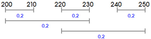
In order to show epistemic uncertainty in evidence theory, a belief structure on input failure strength is constructed as shown in Fig. 4(a), where each interval has a constant BPA of 0.2.

https://cdn.apub.kr/journalsite/sites/jcoseik/2014-027-06/17TK122014270611/images/10.7734.27.6.605.F164.png

https://cdn.apub.kr/journalsite/sites/jcoseik/2014-027-06/17TK122014270611/images/10.7734.27.6.605.F165.png

Figure 4

CBF and CPF of the probability of failure

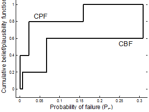
The main process of evidence theory is to find the cumulative belief function(CBF) and the cumulative plausibility function(CPF) of the probability of failure. CBF is the cumulative belief that the uncertain probability of failure P_F is less than a given value y, . Similarly, CPF is the cumulative plausibility that the uncertain probability of failure P_F is less than a given value y, .

CBF and CPF can be found by performing a similar process with the interval analysis method: finding minimum and maximum values and accumulating BPA of each interval. Since the interval analysis method is used for each interval, the evidence theory can be expensive, especially when multiple variables are involved.

Fig. 4(b) shows the CBF and CPF for the probability of failure. Similar to the interval analysis method, it is not easy to define a confidence interval for the evidence theory. However, different from the interval analysis method, it is possible to estimate a narrower interval corresponding to 90 percentile from CBF and CPF graphs. For example, 90 percentile of CBF is 0.15, while that of CPF is 0.309. Therefore, the range of the probability is much narrower than that of the interval analysis method. In addition, this range also covers the 90 percentile from the probability method, =0.23.

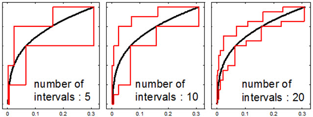
The interpretation of CBF and CPF is a combination of the probability method and the interval analysis method. For example, the minimum likelihood that the probability of failure is less than 0.1 is 0.6, while the maximum likelihood is 0.8. Therefore, connecting with the probability method, it is possible to consider that CBF is the lower-bound of CDF, and CPF is the upper-bound. This observation becomes clear if the number of intervals increases. Fig. 5 compares the CBF and CPF for different number of intervals. It is clear that as the number of intervals increases, the gap between CBF and CPF decreases and both the CBF and CPF converge to the distribution of probability of failure obtained from the probability method (black curve).

https://cdn.apub.kr/journalsite/sites/jcoseik/2014-027-06/17TK122014270611/images/10.7734.27.6.605.F172.png

Figure 5

Comparision between probability method and evidence theory with different numbers of intervals

4. Conclusions

In this paper, four different methods of representing epistemic uncertainty are presented in estimating the uncertainty in the probability of failure. It is found that the probability method represents the uncertainty most accurately as it uses the full distribution of input uncertainty. On the other hand, the interval analysis method only provides a lower- and upper-bounds of the probability of distribution because of the lack of information in input epistemic uncertainty. Since computational costs of these two methods are almost identical, the choice depends on the availability of information of the input uncertainty.

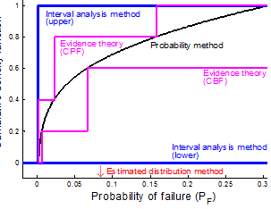
The combined distribution method has a computational advantage but only provides the mean value of the distribution, which can be dangerous especially when the distribution is highly skewed. However, this method is the most computationally inexpensive. The evidence theory is located between the probability method and the interval analysis method, but the computational cost can be the highest among four methods. As more information is available for input uncertainty, this method converges to the probability method. Fig. 6 illustrates the distributions of the probability of failure from the four methods.

https://cdn.apub.kr/journalsite/sites/jcoseik/2014-027-06/17TK122014270611/images/10.7734.27.6.605.F173.png

Figure 6

CDF of the probability of failure

Based on this study, it is concluded that it is important to choose a method based on the level of information available in input epistemic uncertainty.

Acknowledgements

This work is supported by the U.S. Department of Energy, National Nuclear Security Administration, Advanced Simulation and Computing Program, as a Cooperative Agreement under the Predictive Science Academic Alliance Program, under Contract No. DE-NA0002378, and also by the Agency for Defense Development, International Cooperative Research, under contract No. UD130062GD.

Notes

Nomenclature

G : Limit-state function

S : Capacity(failure strength)

R : Response(applied stress)

μ_true : Mean of true failure strength

μ_test : Mean failure strength from test

μ_est : Estimate of true mean failure strength

σ_true : Standard deviation of true failure strength

σ_test: Standard deviation of failure strength from test

σ_est : Estimated standard deviation of true failure strength

References

A.P., Dempster, 1967. Upper and Lower Probabilities Induced by a Multi-valued Mapping. Ann. Mather. Stat., 38, pp.325-339.

10.1214/aoms/1177698950

S., Ferson, C.A., Joslyn, J.C., Helton, W.L., Oberkampf and K., Sentz, 2004. Summary from the Epistemic Uncertainty Workshop: Consensus Amid Diversity. Reliab. Eng. &Syst. Saf., 85, pp.355-369.

10.1016/j.ress.2004.03.023

J.C., Helton and R.J., Breeding, 1993. Calculation of Reactor Accident Safety Goals,. Reliab. Eng. &Syst. Saf., 39, pp.129-158.

10.1016/0951-8320(93)90038-Z

Helton J.C. Johnson J.D. Oberkampf W.L. Sallaberry C.J. 2008Representation of Analysis Results Involving Aleatory and Epistemic UncertaintySandia National Laboratories Technical Report SAND 2008-4379.

10.2172/940535

S., Kari and S, Ferson, 2011. Probabilistic Bounding Analysis in the Quantification of Margins and Uncertainties. Reliab. Eng. &Syst., Saf., 96, pp.1126-1136.

10.1016/j.ress.2011.02.014

C.Y., Park, N.H., Kim and R.T., Haftka, 2014. How Coupon and Element Tests Reduce Conservativeness in Element Failure Prediction. Reliab. Eng. &Syst. Saf., 123, pp.123-136.

10.1016/j.ress.2013.10.012

Shafer G. 1976FA mathematical theory of evidencePrinceton University Press.

Swiler L.P. Paez T.L. Mayes R.L. 2009Epistemic Uncertainty Quantification TutorialProceedings of the 27th International Modal Analysis Conference.

U.S. Department of Defense 2002 Guidelines for Property Testing of CompositesComposite Materials Handbook MIL-HDBK-17.

L.A., Zadeh, 1999. Fuzzy Sets as a Basis for a Theory of Possibility. Fuzzy Sets &Syst., 100, pp.9-23.

10.1016/S0165-0114(99)80004-9

Journal of the Computational Structural Engineering Institute of Korea ISSN:1229-3059(Print) 2287-2302(Online) 한국전산구조공학회 논문집

Preview

Comparison among Methods of Modeling Epistemic Uncertainty in Reliability Estimation

ABSTRACT

MAIN

Figure 1

Illustration of the concept of aleatory and epistemic uncertainty of the failure strength distribution

Table 1

Distribution parameters for aleatory and epistemic uncertainty

Figure 2

Double-loop Monte Carlo simulation for estimated distribution of failure strength

Figure 3

PDF of the probability of failure and its 90 percentile conservative estimate

Table 2

Comparison of uncertainty in the probability of failure between different methods

Figure 4

CBF and CPF of the probability of failure

Figure 5

Comparision between probability method and evidence theory with different numbers of intervals

Figure 6

CDF of the probability of failure

Acknowledgements

Notes

References