Topology Design Optimization of Plate Buckling Problems Considering Buckling Performance

Lee Seung-Wook; Ahn Seung-Ho; Cho Seonho

doi:10.7734/COSEIK.2015.28.5.441

Preview

Journal of the Computational Structural Engineering Institute of Korea. 2015. 441-449
https://doi.org/10.7734/COSEIK.2015.28.5.441

Topology Design Optimization of Plate Buckling Problems Considering Buckling Performance

좌굴성능을 고려한 평판 좌굴문제의 위상설계최적화

Lee Seung-Wook

Ahn Seung-Ho

Cho Seonho^†^*

National Creative Research Initiatives(NCRI) Center for Isogeometric Optimal Design Department of Naval Architecture and Ocean Engineering

• 본 논문에 대한 토의를 2015년 10월 30일까지 학회로 보내주시면 2015년 12월호에 토론결과를 게재하겠습니다.

^*Corresponding Author : seoch@snu.ac.kr

License:

This is an Open-Access article distributed under the terms of the Creative Commons Attribution Non-Commercial License(http://creativecommons.org/licenses/by-nc/3.0) which permits unrestricted non-commercial use, distribution, and reproduction in any medium, provided the original work is properly cited.

ABSTRACT

본 논문에서는 커코프 판이론과 폰-칼만 비선형 변형율-변위 관계를 이용하여 서형화된 좌굴해석을 수행하였다. 평면응력과 좌굴문제에서 영률과 두께에 관한 설계민감도식을 유도하였고, 고유치를 최대화하면서 컴플라이언스를 최소화하는 위상최적설계 기법을 정식화하였다. 좌굴해석에서의 프리스트레스를 이용하여 판 좌굴문제에 적용할 수 있는 위상최적설계 기법을 개발하였다. 폰-칼만 비선형 변형률을 사용하여 좌굴문제의 응력행렬을 구성하는데 프리스트레스가 필요하므로 면외로의 운동을 도입하였다. 위상최적설계를 위하여 정규재료밀도를 설계변수로 하고, 목적함수는 최소 컴플라이언스와 최대 고유진동수로 하였으며 제한조건은 허용되는 재료량이다. 여러 수치예제를 통하여 개발된 설계민감도 해석법은 유한차분 민감도와 비교하여 매우 정확한 값을 가지고, 위상최적설계는 물리적으로 의미있는 결과를 제공함을 확인하였다.

In this paper we perform a linearized buckling analysis using the Kirchhoff plate theory and the von Karman nonlinear strain-displacement relation. Design sensitivity analysis(DSA) expressions for plane elasticity and buckling problems are derived with respect to Young’s modulus and thickness. Using the design sensitivity, we can formulate the topology optimization method for minimizing the compliance and maximizing eigenvalues. We develop a topology optimization method applicable to plate buckling problems using the prestress for buckling analysis. Since the prestress is needed to assemble the stress matrix for buckling problem using the von Karman nonlinear strain, we introduced out-of-plane motion. The design variables are parameterized into normalized bulk material densities. The objective functions are the minimum compliance and the maximum eigenvalues and the constraint is the allowable volume. Through several numerical examples, the developed DSA method is verified to yield very accurate sensitivity results compared with the finite difference ones and the topology optimization yields physically meaningful results.

키워드

설계민감도 해석, 고유치 문제, 좌굴해석, 프리스트레스, 위상최적설계

design sensitivity analysis, eigenvalue, buckling analysis, prestress, topology optimization

MAIN

1. Introduction

The subject of this paper is topology optimization of a buckling problem. A topology optimization method helps designers find a suitable material layout for the required performances. Bendsoe and Kikuchi’s(1988) homogenization based approach was introduced for the topology optimization, and many linear material behaviors and geometrically nonlinear topology optimization methods have been developed (Jung and Cho, 2003). Since the topology optimization necessarily involves many design variables, the design sensitivity analysis(DSA) of performance measure with respect to the design variables should be determined in a very efficient way. A continuum based DSA approach, which can handle several types of design variables, was developed(Haug et al., 2003). In this paper, a continuum method for the non-shape problems like material property is considered. We develop an efficient DSA method for both the maximization of critical load and minimization of compliance.

Buckling may occur as a structural response when the in-plane directional membrane force is applied to the structures. The motion of interest occurs out-of-plane direction because the out-of- plane directional buckling motion occurs faster than the in-plane directional buckling motion. The prestress to be added to the structural forces is one of the forces in the plate. An initial stress matrix is added to the original matrix equation of the structure and consists the buckling equation(Cook et al., 1989). We apply the von Karman strain-displacement relation(Irving et al., 1985) to the original equation to derive the plate buckling equation. The plate buckling topology optimization problems are formulated using the derived plate buckling equation. Finally, the plate buckling topology design optimization problem is performed in several cases.

2. Plate Buckling Problems

The plate buckling governing equation is derived using the von Karman strain- displacement relation and kirchoff plate theory. Next, we can obtain the plate buckling equation as the following:

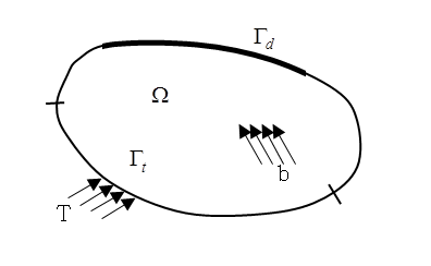
$D \nabla^{4} ω - (N_{x} \frac{\partial^{2} ω}{\partial x^{2}} + {2N}_{x y} \frac{\partial^{2} ω}{\partial x \partial y} + N_{y} \frac{\partial^{2} ω}{\partial y^{2}}) = 0$ (1)

where $\nabla^{4} = (\frac{\partial^{4}}{\partial x^{4}} + 2 \frac{\partial^{4} ω}{\partial x^{2} \partial y^{2}} + \frac{\partial^{4}}{\partial y^{4}})$ and w is the bending deflection. N_x, N_y, N_xy are the forces in the x, y, xy direction measured per unit length shown in Fig. 1 respectively.

https://cdn.apub.kr/journalsite/sites/jcoseik/2015-028-05/01TK102015280501/images/10.7734.28.5.441.F102.png

Figure 1

External force component

Consider a simple built-up structure with domain Ω shown in Fig. 2. The boundary of Ω is composed of Γ_d where the displacement is prescribed and Γ_t where traction t is the prescribed boundary.

https://cdn.apub.kr/journalsite/sites/jcoseik/2015-028-05/01TK102015280501/images/10.7734.28.5.441.F103.png

Figure 2

Elastic body in space

The weak formulation of the fourth order differential Eq. (1) can be obtained by multiplying the virtual bending deflection with it, and integrating the equation over the domain Ω. We obtain Eq. (2) through the integration by part

${\int \int}_{Ω} \frac{D}{2} [\nabla^{2} ω^{2} \bar{ω} + 2 (1 - υ) {(\frac{\partial^{2} ω}{\partial x \partial y}) (\frac{\partial^{2} \bar{ω}}{\partial x \partial y}) -$ (2)

${\frac{\partial^{2} ω}{{\partial x}^{2}} \frac{\partial^{2} \bar{ω}}{{\partial y}^{2}} - \frac{\partial^{2} \bar{ω}}{{\partial x}^{2}} \frac{\partial^{2} ω}{{\partial y}^{2}}}] d Ω + \int}_{Γ} (\frac{\partial \bar{ω}}{\partial n} + Mω + \bar{ω} Nω) d Γ$

${= \frac{1}{2} λ \int \int}_{Ω} {N_{x} (\frac{\partial ω}{\partial x}) (\frac{\partial \bar{ω}}{\partial x}) + N_{y} (\frac{\partial ω}{\partial x}) (\frac{\partial \bar{ω}}{\partial y})$

$N_{y} (\frac{\partial ω}{\partial x}) (\frac{\partial \bar{ω}}{\partial y}) + N_{x y} (\frac{\partial \bar{ω}}{\partial x}) (\frac{\partial \bar{ω}}{\partial y})\} d Ω$

where D is the flexural rigidity and λ is the Critical load factor. M_ω represents the bending moment, and N_ω represents the transverse shear force. The space of kinematically admissible field is defined as a set of displacement field. The space W for the trial solution is defined as

$W = \{ω \in H^{1} (Ω) : ω_{i} = ω_{0} on Γ_{d} i = 1, 2, . . ., r\}$ (3)

Also, space for the virtual displacement field is defined as

$\bar{W} = \{\bar{ω} \in H^{1} (Ω) : \bar{ω_{i}} = 0 on Γ_{d} i = 1, 2, . . ., r\}$ (4)

where r is the number of elements within the built up structure and 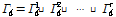is the essential boundary where the displacement is prescribed. By definition, Eq. (4) satisfies for every that belongs to the space of kinematically admissible fields. Due to the above boundary conditions, boundary integrals of Eq. (2) vanish, and variational equation Eq. (2) can be rewritten using bilinear forms as

$a_{Ω} (ω, \bar{ω}) = λ d_{Γ} (ω, \bar{ω}) \forall \bar{ω} \in \bar{ω}$ (5)

The bilinear forms are represented as

$a_{Ω} (ω, \bar{ω}) = \sum_{i = 1}^{r} \int \int_{Ω}^{} \frac{D_{i}}{2} [\nabla^{2} ω_{i} \nabla^{2} \bar{ω} + 2 (1 - υ_{i})$

${(\frac{{\partial^{2} ω}_{i}}{\partial x \partial y}) (\frac{\partial^{2} \bar{ω_{i}}}{\partial x \partial y}) - \frac{{\partial^{2} ω}_{i}}{\partial x^{2}} \frac{\partial^{2} \bar{ω_{i}}}{\partial y^{2}} - \frac{\partial^{2} \bar{ω_{i}}}{\partial x^{2}} \frac{{\partial^{2} ω}_{i}}{\partial y^{2}}}] d Ω$ (6)

and

$d_{Γ} (ω, \bar{ω}) = \sum_{i = 1}^{r} \int \int_{Ω}^{} \frac{1}{2} [N_{x} (\frac{{\partial ω}_{i}}{\partial x}) (\frac{\partial \bar{ω_{i}}}{\partial x}) + N_{y} (\frac{{\partial ω}_{i}}{\partial y}) (\frac{\partial \bar{ω_{i}}}{\partial y})$

$N_{x y} (\frac{{\partial ω}_{i}}{\partial x}) (\frac{\partial \bar{ω_{i}}}{\partial y}) + N_{x y} (\frac{\partial \bar{ω_{i}}}{\partial x}) (\frac{{\partial ω}_{i}}{\partial y})}] d Ω$ (7)

3. Design Sensitivity Analysis of Plate Buckling Problems

Eigenvalue problems for buckling of elastic systems are described by a variational equation form

$a_{u} (ω, \bar{ω}) = {λd}_{u} (ω, \bar{ω}) \forall \bar{ω} \in \bar{W}$ (8)

where satisfies the homogeneous boundary condition and belongs to the space of kinematically admissible displacements. The bilinear form on the right side of Eq. (8) represents geometric effects in buckling problems. A variation of Eq. (8) about the design variable to calculate the design sensitivity is written as

${a^{'}}_{δ u} (ω, \bar{ω}) = a_{u} (ω^{'}, \bar{ω})$

$= λ^{'} d_{u} (ω, \bar{ω}) + λ^{'} d_{δ u} (ω^{'}, \bar{ω}) + λ^{'} d_{u} (ω^{'}, \bar{ω}) \forall \bar{ω} \in \bar{W}$ (9)

where is involved in the variational space, so can be written as w. Then, we obtain

${a^{'}}_{δ u} (ω, \bar{ω}) = a_{u} (ω^{'}, \bar{ω})$

$= λ^{'} d_{u} (ω,ω) + {λ d}^{'}_{δ u} (ω^{'},ω) + λ d_{u} (ω^{'},ω)$ (10)

Design sensitivity of critical buckling load factor λ is written as

λ^' = $\frac{a^{'} d_{u} (ω,ω) + a_{δ u} (ω^{'},ω) - λ {d^{'}}_{u} (ω^{'},ω) - λ d_{u} (ω^{'},ω)}{d_{u} (ω, ω)}$ (11)

$λ^{'} = (ω,δω) = \frac{d}{d τ} [λ (ω + τδω)] |_{τ = 0}$ (12)

Since virtual displacement is involved in variational space, Eq. (11) is rewritten as

$\frac{d λ}{d u} δu = λ^{'} = \frac{a^{'} d_{u} (ω,ω) - λ {d^{'}}_{u} (ω^{'},ω)}{d_{u} (ω,ω)}$ (13)

4. Formulation of Topology Design Optimization

The objective of the topology optimization method is to find an optimal material distribution that minimizes objective functions and is subject to constraints. The material distribution can be represented using a normalized bulk material density function ρ that has a continuous variation from zero to one, taking the value of one for solid material and zero for void. Bulk material density of each element is associated with Young’s modulus and is written as

$E_{i} = ρ_{i}^{p} E_{0}, (i = 1, 2, . . .,N)$ (14)

$0 < ρ_{m i n} \leq ρ_{i} \leq 1$ (15)

where E₀, is the Young’s modulus of the original material.p is a penalty parameter used to enforce a concentrated distribution of material.

4.1 Topology Optimization of Compliance

A topology design optimization without the critical buckling load problem is stated as

Minimize $C = \int \int \int_{Ω}^{} f^{T} z d Ω + \int \int_{Γ_{t}}^{} T^{T} z d Γ_{t}$ (16)

Subject to $V = \int \int \int_{Ω}^{} ρ d Ω \leq V_{0}$ (17)

where C is the compliance, f is the body force intensity,T is the traction, d is the Displacement field, Ω is the structural domain, V₀ is the allowance material volume and ρ is the bulk material density. The sensitivity of design variable for the finite element method is obtained by the variation of Eq. (16) which is written as

$\frac{d C}{d u} = \sum_{k} (\frac{{d f}_{k}}{d u} z_{k} + f_{k} \frac{{d z}_{k}}{d u})$ (18)

The total volume of structure is calculated by design variable ρ_i. The constraint is expressed as

$g = \sum_{i} ρ_{i} V_{i} - V_{0} \leq 0$ (19)

where g is the constraint, ρ_i is the material density and V_i is the volume. We use the Modified Method of Feasible Direction(MMFD) to find the optimal design and MMFD is based on the gradient for the design variables. We need the sensitivity of objective function and the sensitivity of constraint. The sensitivity of constraint is obtained by

$\frac{d g}{d u} \equiv V_{i}$ (20)

4.2 Topology Optimization for Buckling

We formulate the topology optimization considering the critical buckling load. If the compliance is considered only in optimization problem, only the stiffness of the structure can be hardened. Eq. (21) can be obtained by dividing Eq. (16) by the critical buckling load term.

$\bar{C} = \frac{C}{λ_{c}} = \frac{\sum_{k} f_{k} z_{k}}{λ_{c}}$ (21)

Objective function can express both objectives that minimize the compliance and maximize the critical buckling load. We use the allowance material volume as the constraint. The design sensitivity of objective function is written as

$\frac{d \bar{C}}{d u} = \frac{1}{λ_{c}} \frac{d C}{d u} - \frac{1}{λ_{c}} \frac{d λ_{c}}{d u}$ (22)

Using the sensitivities, critical buckling load factor, and compliance, Eq. (22) can be computed.

5. Numerical Examples

5.1 DSA Verification

The purpose of this example is to verify the DSA method for the critical buckling load. We have two results in this numerical example of DSA. The first example is to verify the DSA of the critical buckling load with respect to Young’s modulus and the second example is to verify the DSA of critical buckling load with respect to thickness. The DSA method for the critical buckling load is verified and the buckling mode is made by the axial load and the shear direction load respectively. We use the Kirchhoff plate element to analyze the structure model and use the prestress to calculate the out-of-plane buckling load factor through the plane analysis. We obtain the DSA for critical buckling load applied to these two different type loads, the axial compress force and the shear force.

5.1.1 DSA of Critical Buckling under Axial Compression Force

Consider a square plate whose aspect ratio is 4 under the distribute loading condition as shown in Fig. 3. The rectangular plate is discretized by 16×4 elements. The rectangular plate has a height of 40m, widthof 10m and a plate thickness of 0.01m. A distributive axial compress loading F=1N/m is applied along the right and left sides. Young’s modulus is 209×10⁹(N/m²). Poison’s ratio is ν=0.3. Design variables are relative density and thickness for each element. Performance measure is the critical buckling load.

https://cdn.apub.kr/journalsite/sites/jcoseik/2015-028-05/01TK102015280501/images/10.7734.28.5.441.F139.png

Figure 3

Distributive axial compression applied plate

The analytical design sensitivity of the critical buckling load factor with respect to Young’s modulus is compared with the finite difference sensitivity. In Table 1, design sensitivity of the critical buckling load factor in each nodes with respect to Young’s modulus of each element is compared. We compare the results of analytical sensitivity denoted as dλ/dρ_i with an identical result denoted as ∆λ/∆ρ_i. We compare the exact solution with numerical solution for critical buckling load. They show good agreement shown in Table 2.

Table 1

Comparison of critical buckling load

	Exact solution	Numerical solution	Accuracy(%)
Critical buckling load	7.55584E+03	7.5452E+03	99.856

Table 2

Comparison of design sensitivity

Design Variable			Accuracy(%)
1	6.8516E-10	6.8517E-10	99.99935
2	-2.009E-11	-2.010E-11	99.97837
3	7.8755E-10	7.8761E-10	99.99318
4	8.2416E-10	8.2421E-10	99.99402
9	7.8755E-10	7.8761E-10	99.99319
14	7.3947E-10	7.3939E-10	100.0106
22	6.5191E-10	6.5178E-10	100.0197
28	-2.879E-11	-2.879E-11	99.99806

We use the same way to verify the sizing sensitivity analysis results. The analytical design sensitivity of the critical buckling load with respect to thickness is compared with the finite difference sensitivity. In Table 3, the critical buckling load factor design sensitivity of each node with respect to thickness of each element is compared. We compare the results of analytical sensitivity and the identical result. They show excellent agreement shown in Table 3.Design Variable

Table 3

Comparison of design sensitivity

Design Variable			Accuracy(%)
45	4.15350E+04	4.15268E+04	100.0196
46	3.07400E+04	3.07254E+04	100.0472
47	1.33736E+04	1.33873E+04	99.89730
48	5.56600E+04	5.56554E+04	100.0081
49	5.74150E+04	5.73722E+04	100.0744
50	1.59256E+04	1.59127E+04	100.0812
51	2.94062E+04	2.93863E+04	100.0676
64	5.64241E+04	5.63909E+04	100.0589

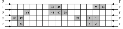
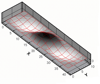
When the axial distributive compression force is applied on the plate, the plate is deformed in the out-of-plane direction. The buckling mode shape in the out-of-plane direction is shown in Fig. 4.

https://cdn.apub.kr/journalsite/sites/jcoseik/2015-028-05/01TK102015280501/images/10.7734.28.5.441.F144.png

Figure 4

Mode shape of axial distributive force applied

5.1.2 DSA of the Critical Buckling Applied the Shear Force

Consider the same model shown in Fig. 5. The rectangular plate is discretized by 16×4 elements. The rectangular plate has a height of 40m, width of 10m and plate thickness of 0.01m. A distributive shear loading, F=1N/m is applied along the edges. Design variables are the relative density for each element. Performance measure is the critical buckling load.

https://cdn.apub.kr/journalsite/sites/jcoseik/2015-028-05/01TK102015280501/images/10.7734.28.5.441.F145.png

Figure 5

Distributive shear loading applied plate

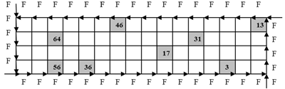
The analytical design sensitivity of the critical buckling load factor with respect to the relative density for each element is compared with the finite difference sensitivity. In Table 4,

Table 4

Comparison of the critical buckling load under shear force

	Exact solution	Numerical solution	Accuracy(%)
Critical buckling load	1.055E+04	1.078E+04	102.2243

design sensitivity of the critical buckling load factor in each nodes with respect to Young’s modulus of each element is compared. We compare the results of analytical sensitivity with an identical result. We compare the exact solution with numerical solution for critical buckling load. They show excellent agreement shown in Table 5.

Table 5

Comparison of design sensitivity for young’s modulus

Design Variable			Accuracy(%)
3	6.851674E-10	6.851718E-10	99.999353
13	-2.0095E-11	-2.0100E-11	99.978375
17	7.875598E-10	7.876134E-10	99.993187
31	8.241626E-10	8.242119E-10	99.994024
36	7.875598E-10	7.876134E-10	99.993190
46	7.394736E-10	7.393946E-10	100.01069
50	6.519138E-10	6.517853E-10	100.01972
64	-2.8791E-11	-2.8791E-11	99.998068

We use the same way to verify the sizing sensitivity analysis result. The analytical design sensitivity of the critical buckling load with respect to thickness is compared with the finite difference sensitivity. In Table 3, the critical buckling load factor design sensitivity of each node with respect to thickness of each element is compared. We compare the results of the analytical sensitivity and an identical result. They show excellent agreement shown in Table 6.

Table 6

Comparison of design sensitivity of thickness

Design Variable			Accuracy(%)
3	5.39079E+04	5.39500E+04	99.922040
13	1.89282E+03	1.89468E+03	99.901825
17	5.53565E+04	5.52252E+04	100.23774
31	9.96608E+04	9.95562E+04	100.10505
36	5.44183E+04	5.43790E+04	100.07223
46	1.36546E+04	1.36098E+04	100.32954
50	3.66279E+03	3.65487E+03	100.21656
64	3.68065E+04	3.66810E+04	100.34209

When the shear distributive force is appliedto the plate, the plate is deformed in the out-of-plane direction. The buckling mode shape in the out-of- plane direction is shown in Fig. 6.

https://cdn.apub.kr/journalsite/sites/jcoseik/2015-028-05/01TK102015280501/images/10.7734.28.5.441.F147.png

Figure 6

Mode shape of distributed shear force applied

5.2 Topology Optimization

5.2.1 Topology optimization Applied the Axial Compression Force

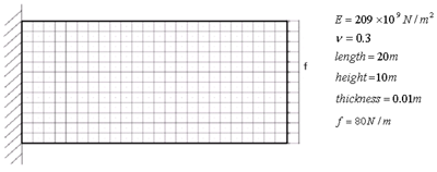
The cantilever model subjected to a distributive axial compression is shown in Fig. 7. The optimization result without considering the critical buckling load is also shown in Fig. 8 and the buckling mode shape is shown in Fig. 9. The critical buckling load factor is the value to multiply to the initial loading. In this example the critical buckling load factor is 0.392977.

https://cdn.apub.kr/journalsite/sites/jcoseik/2015-028-05/01TK102015280501/images/10.7734.28.5.441.F148.png

Figure 7

Cantilever model specification under axial compression

https://cdn.apub.kr/journalsite/sites/jcoseik/2015-028-05/01TK102015280501/images/10.7734.28.5.441.F149.png

Figure 8

Optimal shape without considering buckling

https://cdn.apub.kr/journalsite/sites/jcoseik/2015-028-05/01TK102015280501/images/10.7734.28.5.441.F150.png

Figure 9

Buckling mode without considering buckling

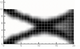
The topology optimization results considering the critical buckling load is shown in Fig. 10 and the buckling mode shape is shown in Fig. 11. In this case, the critical buckling load factor is 0.534326. The critical buckling load factor increased 36% than the previous result. We can modify the layout performance of the critical buckling load.

https://cdn.apub.kr/journalsite/sites/jcoseik/2015-028-05/01TK102015280501/images/10.7734.28.5.441.F151.png

Figure 10

Optimal shape with considering buckling

https://cdn.apub.kr/journalsite/sites/jcoseik/2015-028-05/01TK102015280501/images/10.7734.28.5.441.F152.png

Figure 11

Buckling mode with considering buckling

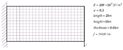
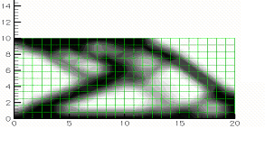
5.2.2 Topology optimization under shear force

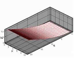
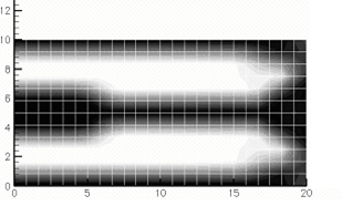
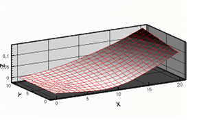
The cantilever model subjected to a distributed shear force is shown in Fig. 12. The final material distribution after the topology optimization result except for considering the critical buckling load is also shown in Fig. 13 and the buckling mode shape is shown in Fig. 14. The critical buckling load factor is 2.401125.

https://cdn.apub.kr/journalsite/sites/jcoseik/2015-028-05/01TK102015280501/images/10.7734.28.5.441.F153.png

Figure 12

Cantilever model specification under shear force

https://cdn.apub.kr/journalsite/sites/jcoseik/2015-028-05/01TK102015280501/images/10.7734.28.5.441.F154.png

Figure 13

Optimal shape without considering buckling

https://cdn.apub.kr/journalsite/sites/jcoseik/2015-028-05/01TK102015280501/images/10.7734.28.5.441.F155.png

Figure 14

Buckling mode shape without considering buckling

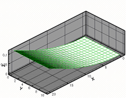
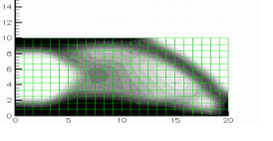
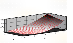
The topology optimization results considering the critical buckling load is shown in Fig. 15 and the buckling mode shape is shown in Fig. 16. The critical buckling load factor is 2.727772 in this case. The critical buckling load factor increased 14% than the previous result. We can modify the layout performance of the critical buckling load.

https://cdn.apub.kr/journalsite/sites/jcoseik/2015-028-05/01TK102015280501/images/10.7734.28.5.441.F156.png

Figure 15

Optimal shape with considering buckling

https://cdn.apub.kr/journalsite/sites/jcoseik/2015-028-05/01TK102015280501/images/10.7734.28.5.441.F157.png

Figure 16

Buckling mode shape with considering buckling

6. Conclusion

We derive the plate buckling equation including the out-of-plane direction buckling motion. Based on this equation, we derive a weak formulation for plate buckling problems and a continuum-based DSA method using a direct differentiation for eigenvalue design sensitivity approach in continuum form. Also, a topology design optimization method for plate buckling problems using the Kirchhoff plate theory is developed using the direct DSA method. For the topology optimization, the displacement of the buckling motion is calculated. The design variables are parameterized using bulk material densities.

Through several numerical examples, we verify the accuracy of the analytical DSA method by comparing the finite difference sensitivity. The analytical DSA method yields very accurate sensitivity results compared with those of the central finite difference method. Also the topology optimization yields physically meaningful results. It could result in different optimal shapes depending on the critical buckling load and force applied. The topology optimization results considering the critical buckling load factor significantly increase the critical buckling load factor.

Acknowledgements

This work was supported by the National Research Foundation of Korea(NRF) grant funded by the Korea government(No.2010-0018282). The support is gratefully acknowledged. The authors would also like to thank Ms. Inyoung Cho at Korea University for editing assistance.

References

M.P., Bendsøe and N., Kikuchi, 1988. Generating Optimal Topologies in Structural Design using a Homogenization Method. Comput. Methods Appl. Mech & Eng., 71, pp.197-224.

10.1016/0045-7825(88)90086-2

Cook R.D. Malkus D.S. Plesha M.E. 1989Concepts and Applications of Finite Element AnalysisJohn Wiley & Sons Inc784

E.J., Haug, K.K., Choi and V., Komkov, 1986. Design Sensitivity Analysis of Structural System. Academic Press : New York, NY, p.38.

Ha Y.D. Kwak J.H. Cho S. 2002Topology Optimization of Structural Frame in Human Powered VesselProceeding of the Annual Autumn Meeting-SNAK.

Irving H.S. Dym C.L. 1985Energy and Finite Element Method in Structural MechanicsHemisphere Publishing Company776

Jung H.S. 2003Design Sensitivity Analysis and Topology Optimization of Displacement-loaded Nonlinear StructuresComput. Methods in Appl. Mech. & Eng.25392553

M.G., Kim, J.H., Kim and S., Cho, 2010. Topology Design Optimization of Heat Conduction Problems using Adjoint Sensitivity Analysis Method. J. Comput. Struct. Eng. Inst. Korea, 23, pp.683-691.

L.E., Malvern, 1969. Introduction to The Mechanics of a Continuous Medium. Prentice Hall Inc., New Jersey, p.711.

Reddy J.N. 1993An Introduction to The Finite Element MethodMcgraw-Hill Book Company896

Timoshenko S.P. Gere J.M. 1961Theory of Elastic StabilityMcgraw-Hill Book Company541

Timoshenko S.P. Woinowsky K.S. 1987Theory of Plates and ShellsMcgraw-Hill Book Company580

Zienkiewiez O.C. Taylor R.L. 1988The finite Element MethodMcgraw-Hill Book Company,732

Journal of the Computational Structural Engineering Institute of Korea ISSN:1229-3059(Print) 2287-2302(Online) 한국전산구조공학회 논문집

Preview

Topology Design Optimization of Plate Buckling Problems Considering Buckling Performance

ABSTRACT

MAIN

Figure 1

External force component

Figure 2

Elastic body in space

Figure 3

Distributive axial compression applied plate

Table 1

Comparison of critical buckling load

Table 2

Comparison of design sensitivity

Table 3

Comparison of design sensitivity

Figure 4

Mode shape of axial distributive force applied

Figure 5

Distributive shear loading applied plate

Table 4

Comparison of the critical buckling load under shear force

Table 5

Comparison of design sensitivity for young’s modulus

Table 6

Comparison of design sensitivity of thickness

Figure 6

Mode shape of distributed shear force applied

Figure 7

Cantilever model specification under axial compression

Figure 8

Optimal shape without considering buckling

Figure 9

Buckling mode without considering buckling

Figure 10

Optimal shape with considering buckling

Figure 11

Buckling mode with considering buckling

Figure 12

Cantilever model specification under shear force

Figure 13

Optimal shape without considering buckling

Figure 14

Buckling mode shape without considering buckling

Figure 15

Optimal shape with considering buckling

Figure 16

Buckling mode shape with considering buckling

Acknowledgements

References