A MATLAB Implementation of ES-FEM-based Topology Optimization

Changkye Lee

doi:10.7734/COSEIK.2025.38.6.371

Preview

Research Paper

Journal of the Computational Structural Engineering Institute of Korea. 31 December 2025. 371-379
https://doi.org/10.7734/COSEIK.2025.38.6.371

A MATLAB Implementation of ES-FEM-based Topology Optimization

MATLAB으로 구현한 에지 기반 평활화 유한요소법을 도입한 위상 최적화

Changkye Lee¹^*

이 창계¹^*

¹Postdoctoral Research Associate, Division of Cardiovascular Medicine, University of Miami, FL, 33136, USA

¹미국 마이애미대학교 의과대학 박사후연구원

^{*Corresponding Author}

License (open-access, https://creativecommons.org/licenses/by-nc/4.0/):

This is an Open-Access article distributed under the terms of the Creative Commons Attribution Non-Commercial License (https://creativecommons.org/licenses/by-nc/4.0) which permits unrestricted non-commercial use, distribution, and reproduction in any medium, provided the original work is properly cited.

ABSTRACT

This paper presents a compact and efficient MATLAB implementation of topology optimization using the edge-based smoothed finite element method (ES-FEM). The framework is designed with pedagogical intent, illustrating how ES-FEM can be effectively vectorized through the systematic construction of smoothing domains around interior and boundary edges, followed by the computation of smoothed stiffness matrices over these domains. Computational efficiency is further enhanced through array preallocation. An improved density filter is incorporated, simplifying the formulation while delivering better performance compared to existing ES-FEM-based topology optimization approaches. With this enhancement, the complete implementation requires only 175 lines of MATLAB code, ensuring both readability and ease of use. Boundary conditions and loading can be customized by modifying only a few lines, making the approach flexible and easily extensible. The full MATLAB code is provided in the Appendix as an accessible starting point for newcomers to topology optimization and ES-FEM, offering a clear and approachable entry point with a gentle learning curve.

Keywords

topology optimization

smoothed finite element method

MATLAB code

education

본 논문은 에지 기반 평활화 유한요소법(Edge-based smoothed finite element method, ES-FEM)을 도입한 위상 최적화를 간결하고 효율적인 MATLAB 코드로 구현하였다. 제안한 MATLAB 코드는 교육적 목적을 위해 내부 및 경계 에지를 중심으로 평활화 영역을 체계적으로 생성하고, 해당 영역에 대한 평활화 강성 행렬을 계산함으로써 ES-FEM을 효과적으로 벡터화하는 방법을 보여준다. 특히 배열 사전 할당을 통해 계산 효율성을 한층 향상시켰다. 아울러, 개선된 밀도 필터를 도입하여 기존 ES-FEM 기반 위상 최적화 기법보다 수식을 단순화하면서도 계산 성능을 크게 향상시켰다. 이러한 개선으로 전체 MATLAB 코드는 175줄로 구현되어 높은 가독성과 사용 편의성을 갖춘다. 또한 경계 조건과 하중의 적용은 몇 줄만 수정하면 되어, 연구자가 손쉽게 코드를 유연하게 확장할 수 있다. MATLAB 코드는 부록에 수록되어 있으며, 이를 통해 위상 최적화와 ES-FEM에 입문하는 연구자들이 보다 쉽게 학습할 수 있도록 명확하고 직관적인 교육적 자료를 제공하고자 한다.

키워드

위상 최적화

평활화 유한요소법

Matlab 코드

교육용

MAIN

1. Introduction
2. Topology Optimization
3. Edge-based Smoothed Finite Element Method
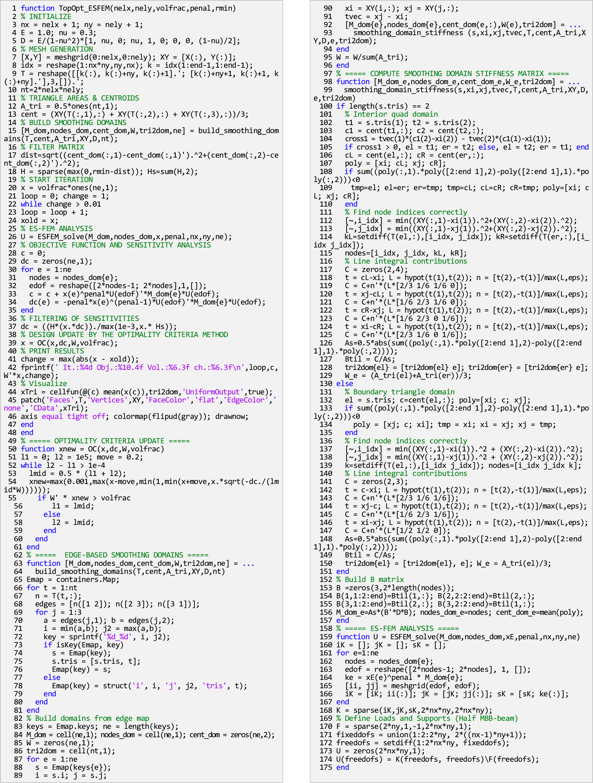
4. MATLAB Implementation
4.1 Main program
4.2 Optimality Criteria solver
4.3 Sensitivity filter
4.4 Edge-based S-FEM code
4.5 MALTAB code extensions
5. Conclusion

1. Introduction

MATLAB is an interpreted programming language and numerical computing environment widely used in engineering, science, economics, and related fields (MathWorks, 2025). Although it is generally less computationally efficient than lower-level languages such as C++ or Fortran for large-scale problems, MATLAB offers extensive built-in functions, specialized toolboxes, and powerful visualization capabilities. Consequently, it remains highly popular for teaching, rapid prototyping, and validation. In structural topology optimization, in particular, MATLAB is frequently used in educational settings because it enables concise and readable implementations that are well suited for instructional purposes.

Topology optimization has become an effective design strategy across diverse engineering applications, aiming to identify optimal material distributions within a design domain subject to physical and geometric constraints (Lee, 2003). Building on Sigmund’s (2001) pedagogical MATLAB implementation, which introduced a concise, problem-oriented code, numerous MATLAB-based approaches using the finite element method (FEM) have since been developed. These include further code simplification (Andreassen et al., 2011), evolutionary structural optimization (Huang and Xie, 2010), level-set methods (Challis, 2010), polygonal meshes (Talischi et al., 2012), and three-dimensional formulations (Liu and Tovar, 2014). Additionally, MATLAB-based topology-optimization codes are available for the geometrically nonlinear structures (Chen et al., 2019), the finite-volume method (Araujo et al., 2024), body-fitted meshing (Zhuang et al., 2024), and thermomechanical loading with steady-state heat conduction (Ooms et al., 2023).

Most MATLAB-based topology optimization studies employ FEM with four-node quadrilateral (Q4) elements because Q4 formulations are algebraically simple, align naturally with MATLAB’s matrix-oriented data structures, and support highly vectorized assembly and filtering routines, thereby keeping both research and teaching codes concise and efficient.

As an extension of conventional FEM-based topology optimization, the smoothed finite element method (S-FEM) with three-node triangular (T3) meshes has been explored (Lee et al., 2021, 2022). Compared with standard FEM, certain S-FEM variants often achieve higher accuracy for a given number of degrees of freedom and tend to produce clearer, less noisy layouts (Liu and Trung, 2016). Benchmark studies have reported comparable or improved compliance reduction with smoother material boundaries. However, S-FEM is typically less computationally efficient: assembling smoothed contributions and forming the global stiffness matrix increase bandwidth and fill-in, thereby raising memory demands and solution time.

To address these trade-offs, this study introduces the edge-based smoothed finite element method (ES-FEM) into density-based topology optimization and implements it in MATLAB, following the concise style of Sigmund’s 99-line code. The goal is pedagogical: to provide a compact instructional tool for learners of both topology optimization and ES-FEM. As a reference framework, the Solid Isotropic Material with Penalization (SIMP) model is employed together with an Optimality Criteria (OC) update scheme, and the density filter of Andreassen et al. (2011) is incorporated to improve robustness and reduce mesh dependence. The main contribution is a simplified procedure for constructing edge-based smoothing domains in both interior and boundary regions and assembling the corresponding smoothed stiffness matrix. With this approach, the ES-FEM topology optimization solver is realized in just 175 lines of MATLAB, maintaining conciseness while improving clarity and computational efficiency.

The paper is organized as follows: Section 2 reviews the formulation of density-based topology optimization and Section 3 summarizes ES-FEM. Section 4 describes the MATLAB implementation and extensions to boundary conditions, multiple load cases, and heat conduction. Section 5 presents observations and discussion

2. Topology Optimization

In topology optimization, the objective is to minimize the structural compliance $c (x)$ subject to standard constraints, expressed as:

(1)

\begin{matrix} \min_{x} : & c (x) = U^{T} \bar{K} U = \sum_{e = 1}^{N_{SD}} x_{e}^{p} U_{e}^{T} {\bar{K}}_{e} U_{e} \\ subject to & \frac{V (x)}{V_{0}} = V_{f} \\ \bar{K} U = F \\ 0 < x_{\min} \leq x \leq 1 \end{matrix}

where $x$ is the vector of design variables, $\bar{K}$ is the global edge-based smoothed stiffness matrix, U is the global displacement vector, and F is the global force vector. The terms ${\bar{K}}_{e}$ and $U_{e}$ denote the smoothed stiffness matrix and displacement vector associated with the e-th smoothing domain, respectively. The lower bound $x_{\min}$ is a small positive constant introduced to prevent singularity, and the penalization power $p$ =3 is utilized in this study. Moreover, $V (x)$ denotes the material volume, $V_{0}$ is the design domain volume, and $V_{f}$ is the prescribed volume fraction.

The optimization problem defined in Eq. (1) is solved using the OC method, with the heuristic updating scheme given by:

(2)

x_{e}^{new} = \{\begin{cases} \begin{array}{ll} max (x_{min}, x_{e} - m) & x_{e} B_{e}^{η} \leq max (x_{min}, x_{e} - m) \end{array} \\ \begin{array}{ll} min (1, x_{e} + m) & x_{e} B_{e}^{η} \leq min (1, x_{e} + m) \end{array} \\ \begin{array}{ll} x_{e} B_{e}^{η} & otherwise \end{array} \end{cases}

where $m$ =0.2 is the move limit and 𝜂=1/2 is the numerical damping coefficient. The coefficient $B_{e}$ in Eq. (2) is derived from the optimality condition as:

(3)

B_{e} = \frac{- \frac{\partial c}{\partial x_{e}}}{λ \frac{\partial V}{\partial x_{e}}}

where 𝜆 is the Lagrange multiplier, determined iteratively using a bisection algorithm.

The sensitivity of the objective function with respect to the design variable of smoothing domain $e$ is:

(4)

\frac{\partial c}{\partial x_{e}} = - p x_{e}^{p - 1} U_{e}^{T} {\bar{K}}_{e} U_{e}

To improve robustness, Eq. (3) is modified by applying a sensitivity filter, expressed as:

(5)

\frac{\partial \hat{c}}{\partial x_{e}} = \frac{1}{\max (γ, x_{e}) \sum_{i \in N_{S D}} H_{e i}} \sum_{i \in N_{S D}} H_{e i} x_{i} \frac{\partial c}{\partial x_{i}}

where 𝛾=10^-3, and $N_{S D}$ denotes the set of smoothing domains $i$ whose centroid-to-centroid distance $∆ (e, i)$ from domain $e$ is smaller than the filter radius $r_{\min}$ . The weighting function $H_{e i}$ is defined as:

(6)

H_{e i} = \max (0, r_{\min} - Δ (e, i))

Eq. (5) and (6) represent one of the main differences from Sigmund(2001), contributing to both improved computational efficiency and a simplification of the MATLAB implementation.

3. Edge-based Smoothed Finite Element Method

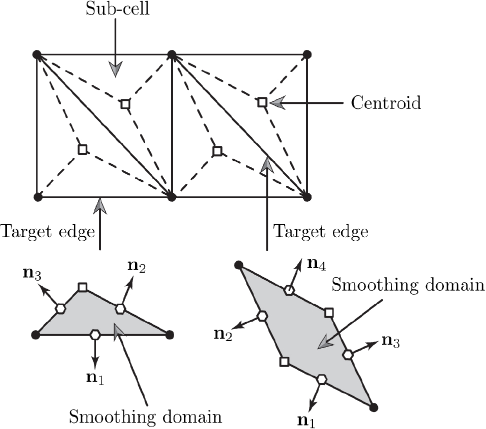
This section briefly revisits the fundamental concept of ES-FEM. The main distinction from the standard FEM is that: (a) each element is subdivided into sub-cells; (b) these sub-cells are rebuilt to form smoothing domains; and (c) the stiffness matrix is evaluated over the smoothing domains rather than the original elements. In ES-FEM, smoothing domains are constructed along the edges of T3 elements together with their adjacent sub-cells, as illustrated in Fig. 1.

https://cdn.apub.kr/journalsite/sites/jcoseik/2025-038-06/N0040380603/images/Figure_jcoseik_38_06_03_F1.jpg

Fig. 1.

Construction of the edge-based smoothing domain

The infinitesimal strain over each smoothing domain $Ω_{k}$ is defined as:

(7)

\bar{ε} (x_{k}) = \int_{Ω_{k}} ε^{h} (x) Φ (x) d Ω

where $x_{k}$ denotes a representative point on the boundary of smoothing domain, and $ε^{h} (x)$ is the compatible strain field.

The weight function $Φ (x)$ is introduced such that:

(8)

\int Φ (x) d Ω = 1 Φ (x) = \{\begin{cases} 1 / A_{k} x \in Ω_{k} \\ 0 x \notin Ω_{k} \end{cases}

where $A_{k}$ is the area of smoothing domain $Ω_{k}$ . By applying divergence theorem to Eq. (7) and using Eq. (8), the smoothed strain can be expressed as:

(9)

\bar{ε} (x_{k}) = \frac{1}{A_{k}} \int_{Ω_{k}} ε^{h} (x) d Ω = \frac{1}{A_{k}} \int_{Γ_{k}} L_{n} (x) u^{h} (x) d Γ

where $L_{n} (x)$ denotes the two-dimensional matrix form of the outward normal vector on boundary $Γ_{k}$ of the smoothing domain.

From Eq. (9), the smoothed strain-displacement matrix is obtained as:

(10)

{\bar{B}}_{I} = \frac{1}{A_{k}} \int_{Γ_{k}} L_{n} (x) ψ_{I} (x) d Γ = [\begin{matrix} {\tilde{b}}_{I x} & 0 \\ 0 & {\tilde{b}}_{I y} \\ {\tilde{b}}_{I y} & {\tilde{b}}_{I x} \end{matrix}] {\tilde{b}}_{I x} = \frac{1}{A_{k}} \int_{Γ_{k}} n_{n} (x) ψ_{I} (x) d Γ

where $h \in {x, y}$ and $ψ_{I} (x)$ is the shape function associated with node $I$ .

The smoothed stiffness matrix using Eq. (10) is then assembled as:

(11)

\bar{K} = \sum_{k = 1}^{N_{S D}} \int_{Ω_{k}} {\bar{B}}^{T} (x) ℂ \bar{B} (x) d Ω_{k} = \sum_{k = 1}^{N_{S D}} \int_{Ω_{k}} {\bar{B}}^{T} (x) ℂ \bar{B} (x) A_{k}

where $ℂ$ is the two-dimensional linear constitutive matrix. The external force vector is computed in the same manner as in the standard FEM. In addition, Eq. (11) is also employed in evaluating the sensitivity of the objective function given in Eq. (4).

4. MATLAB Implementation

The proposed ES-FEM for structural topology optimization is implemented in MATLAB, as provided in Appendix A. The code can be executed as a user-defined function by entering the following command in the MATLAB command window:

TopOpt_ESFEM(nelx,nely,volfrac,penal,rmin)

where nelx and nely are the number of elements in $x$ - and $y$ -directions, volfrac is the prescribed volume fraction, penal is the penalization power, and rmin is the filter size.

4.1 Main program

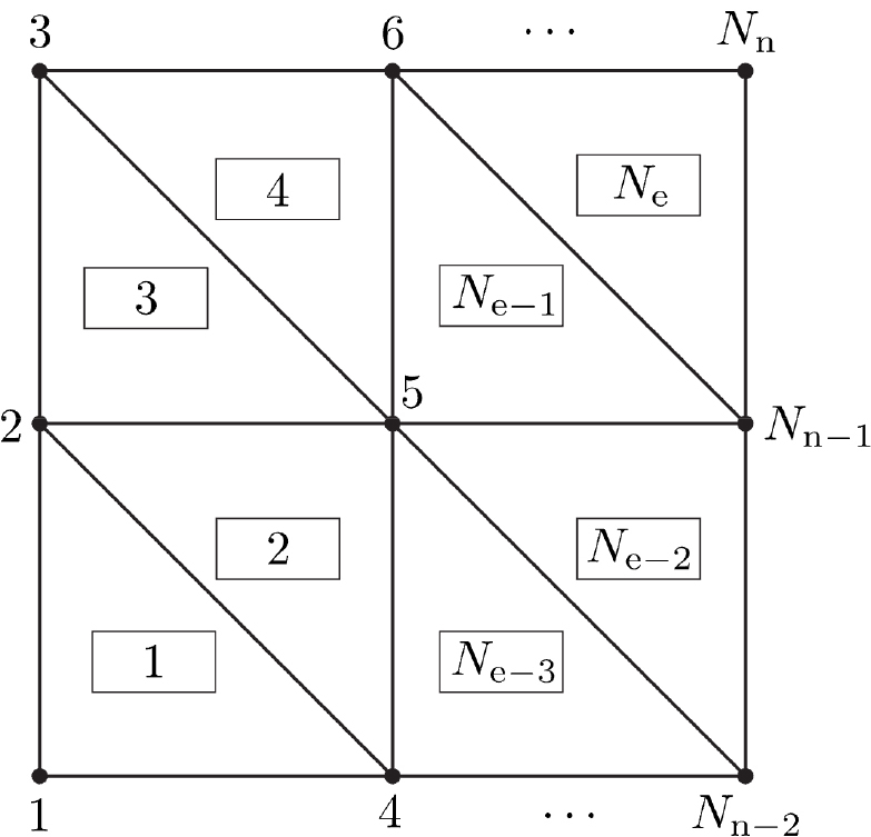
The main program (Lines 1-48) begins with the constitutive matrix under the plane stress assumption (Lines 4-5), followed by the generation of triangular meshes for the rectangular domain (Lines 6-10). In this implementation, each triangular element has unit base and height; thus, the number of elements along the $x$ - and $y$ -directions directly correspond to the geometric dimensions of the domain. The nodes and element numbering convention used in this code is illustrated in Fig. 2.

https://cdn.apub.kr/journalsite/sites/jcoseik/2025-038-06/N0040380603/images/Figure_jcoseik_38_06_03_F2.jpg

Fig. 2.

Discretization of the problem domain into triangular elements with node and element numbering

Once the mesh is generated, the edge-based smoothing domains for both interior and boundary regions are constructed, and the smoothed stiffness matrices are precomputed (Line 15). The optimization loop (Lines 22-47) follows, beginning with the solution of the equilibrium equations (Line 26) to obtain the global displacement vector U.

The objective function and its sensitivity are evaluated on each smoothing domain (Lines 28-35). Sensitivity filtering is applied in Line 37, and the Optimality Criteria (OC) update is performed in Line 39.

During each iteration, compliance, volume fraction, and the maximum change in design variables are printed (Line 42), while the current density distribution is visualized (Lines 44-46). The optimization process terminates once the maximum change in the design variables falls below 0.01.

4.2 Optimality Criteria solver

Design variable updates are performed using the OC method (Lines 50-61). The implementation closely follows the OC function in Sigmund (2001), with the only modification being the inclusion of the smoothing domain weight vector W in the update rule:

xnew=max(0.001,max(x-move,min(1,min(x+move,x.*sqrt(-dc./(lmid*W))))));

A bisection search adjusts the Lagrange multiplier 𝜆 until the prescribed volume fraction is satisfied, while simultaneously enforcing move limits (± 0.2) and design bounds [0.001,1].

4.3 Sensitivity filter

A sensitivity filter based on Eq. (5) is adopted from Andreassen et al. (2011). The filter computes a weighted average of sensitivities across neighboring smoothing domains, thereby reducing numerical instabilities and mesh dependence. In the code, the filter is initialized in Lines 17-18, where pairwise distances between domain centroids are calculated, and the sparse weight matrix H=max(0,rmin-dist) is assembled along with its row-sum vector Hs=sum(H,2). Here, H stores the distance-based weights, while Hs ensures normalization. During the optimization loop, the filtered sensitivities are evaluated in Line 37 as:

dc = ((H*(x.*dc))./max(1e-3,x.*Hs))

In this expression, x.*dc represents the weighted sensitivities, multiplication by H accumulates contributions from neighboring domains, and division by x.*Hs normalizes the sum. The safeguard max(1e-3,x.*Hs) prevents division by very small numbers. This procedure ensures that each design variable is smoothly influenced by its neighbors, resulting in stable convergence and improved robustness of the optimization.

4.4 Edge-based S-FEM code

The core ES-FEM routines are implemented in Lines 62-157, where smoothing domains are constructed along element edges and the corresponding smoothed stiffness matrices are computed. Detection of interior and boundary edges is performed using an edge map in Lines 65-81. Each triangular element contributes three edges that are stored in a map structure; edges shared by two adjacent triangles form interior domains, while edges belonging to a single triangle form boundary domains.

For each domain, the polygon is assembled from the edge endpoints and centroids. Its orientation is checked and corrected using the shoelace formula and the area is evaluated (Lines 100-111 and 131-135):

poly = [xi; cL; xj; cR];

if shoelace(poly)<0, poly=[xi; cR; xj; cL]; end

As=0.5*abs(shoelace(poly));

Outward unit normals along polygon edges are integrated in closed form, giving the coefficients ${\tilde{b}}_{I h}$ in Eq. (10) (Lines 116-125 and 140-147):

t = cL-xi; L = hypot(t(1),t(2));

n = [t(2),-t(1)]/max(L,eps);

C = C+n'*(L*[2/3 1/6 1/6 0]); Btil = C/As;

These coefficients are then used to assemble the smoothed strain-displacement matrix $B$ , and the local stiffness matrix is computed as $M_{dom}^{(e)} = A_{s} (B^{T} ℂB)$ (given in Eq. (11)) implemented in Lines 152-156:

(1,1:2:end)=Btil(1,:); B(2,2:2:end)=Btil(2,:);

B(3,1:2:end)=Btil(2,:); B(3,2:2:end)=Btil(1,:);

M_dom_e=As*(B'*D*B);

Interior domains are assigned to an average area weight $(A_{L} + A_{R}) / 3$ , while boundary domains use $A / 3$ . This closed-form design eliminates the need for numerical quadrature, keeping the implementation concise while remaining directly linked to the ES-FEM formulation. Global assembly of the smoothed stiffness matrices is performed in a domain-wise loop, after which boundary conditions and external loads are applied, and the systems is solved in the same as in Sigmund (2001).

4.5 MALTAB code extensions

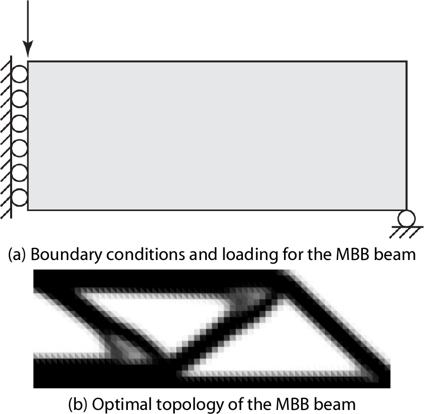
4.5.1 Messerschmitt-Bölkow-Blohm (MBB)

The present code is first demonstrated on the classical Messerschmitt-Bölkow-Blohm (MBB) beam problem using:

TopOpt_ESFEM(60,20,0.5,3,1.5)

and the resulting optimal topology is presented in Fig. 3.

https://cdn.apub.kr/journalsite/sites/jcoseik/2025-038-06/N0040380603/images/Figure_jcoseik_38_06_03_F3.jpg

Fig. 3.

Topology optimization of the MBB beam

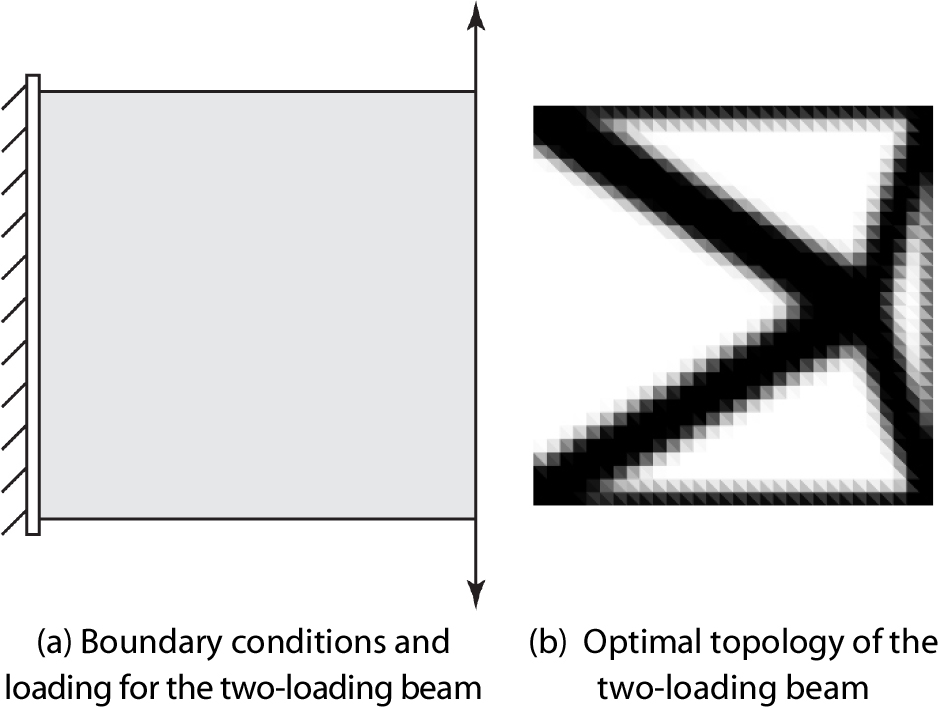
4.5.1 Multiple loading beam

The first extension addresses multiple load cases. In this study, two independent loadings are applied, with the corresponding boundary conditions and external forces are illustrated in Fig. 4(a). For this case, the force and displacement vectors must be defined with two columns, which requires modifying Lines 170-173 as follows:

F = sparse(2*nx*ny,2);

F(2*nx*ny,1) = 1;

F(2*(nx-1)*ny+2,2) = -1;

fixeddofs = 1:2*ny;

freedofs = setdiff(1:2*nx*ny, fixeddofs);

U = zeros(2*nx*ny,2);

https://cdn.apub.kr/journalsite/sites/jcoseik/2025-038-06/N0040380603/images/Figure_jcoseik_38_06_03_F4.jpg

Fig. 4.

Topology optimization of the multiple loading beam

Since the objective function must now account for the sum of the two compliances, Lines 33-34 are replaced by the following loop:

for i=1:2

c = c + x(e)^penal*U(edof,i)'*M_dom{e}*U(edof,i);

dc(e) = dc(e) -

penal*x(e)^(penal-1)*U(edof,i)'*M_dom{e}*U(edof,i);

end

Using these modifications, and with the chosen input parameters, the optimal topology for the two-load case is obtained with:

TopOpt_ESFEM(30,30,0.4,3,1.2)

as shown in Fig. 4(b).

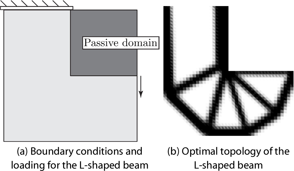
4.5.2 Passive domain

In some optimization problems, certain regions are constrained to remain at a minimum density. A common example is the presence of a passive domain, such as a hole or an excluded region within the design space. To demonstrate this feature, an L-shaped beam with a passive domain located in the top-right corner of the square design domain is considered (Fig. 5(a)). To enforce the minimum density in passive elements, the following line needs to be inserted before the start of the optimization loop: x(passive==1)=0.001;. Passive elements are defined, and the boundaries of the passive domain are detected, by replacing the smoothing-domain construction call in Line 15 with: [M_dom,nodes_dom,cent_dom,W,tri2dom,passive,ne]=build_smoothing_domains(T,cent,A_tri,XY,D,nt,nelx,nely);. In this modified function, the active-passive interface is handled carefully: edges along the passive boundary are treated as boundary domains on the active side only, ensuring that passive flags and associated weights are defined consistently.

https://cdn.apub.kr/journalsite/sites/jcoseik/2025-038-06/N0040380603/images/Figure_jcoseik_38_06_03_F5.jpg

Fig. 5.

Topology optimization of the L-shaped beam with a passive domain

For this case, the force and displacement vectors are defined as two-column vectors, requiring the following modification of Lines 170-172:

F = sparse(2*nx*ny,2);

F(2*nx*ny,1) = 1;

F(2*(nx-1)*ny+2,2) = -1;

fixeddofs = 1:2*ny;

freedofs = setdiff(1:2*nx*ny, fixeddofs);

U = zeros(2*nx*ny,2);

The passive-domain example is solved using:

TopOpt_ESFEM(40,40,0.3,3,1.3)

The resulting optimal topology is shown in Fig. 5(b). Compared with the standard case, the passive region in the top-right corner remains fixed at the minimum density throughout optimization, effectively constraining the design space. This alters the load path and redistributes material around the excluded region, demonstrating that the code can accommodate geometric restrictions.

The fully updated MATLAB functions for defining active-passive smoothing domains and computing the associated smoothed stiffness matrices are available at: https://sourceforge.net/projects/topopt-esfem/files/

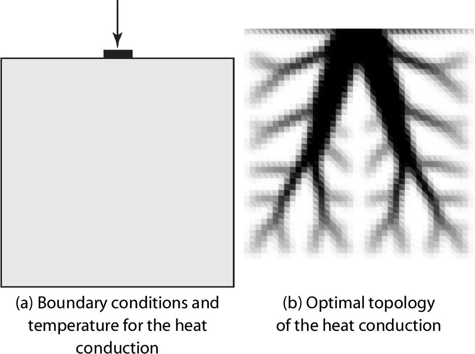
4.5.3 Heat conduction

This final extension addresses heat-conduction topology optimization. A Dirichlet boundary condition is applied at (and immediately around) the midpoint of the top boundary (Fig. 6(a)) with prescribed temperature $T$ =0℃; the remaining boundaries are insulated (zero flux). In the code, the solid/void conductivities and the isotropic conductivity matrix are set in Line 4-5 as:

k0 = 1; kmin = 1e-3;

D = k0*eye(2);

https://cdn.apub.kr/journalsite/sites/jcoseik/2025-038-06/N0040380603/images/Figure_jcoseik_38_06_03_F6.jpg

Fig. 6.

Topology optimization of the heat conduction

A uniform volumetric heat source is applied throughout the domain, and the Dirichlet anchor is enforced by fixing a small stencil of nodes around the top-midpoint for numerical stability:

F = sparse(0.01*ones(nx*ny,1));

mid_x = round((nx-1)/2);

fixeddofs = [(mid_x+1)*nx-ny, (mid_x+1)*ny, (mid_x+1)*nx+ny];

freedofs = setdiff(1:nx*ny,fixeddofs);

U = zeros(nx*ny,1);

Because temperature is a scalar quantity per node, each domain’s smoothed matrix is taken directly as B=Btil; (no Voigt expansion), replacing Lines 153-156 in smoothing_domain_stiffness with the scalar form and adjusting node indices accordingly. Material interpolation follows the standard SIMP law for conductivity, $k (x_{e}) = k_{\min} + (1 - k_{\min}) x_{e}^{p}$ , which is applied in both the stiffness matrix and the sensitivity. Thus, Lines 32-34 are replaced with:

edof = node_dom{e};

c = c +

(kmin+(1-kmin)*x(e)^penal)*U(edof)'*M_dom{e}*U(edof);

dc(e) = -penal*(1-kmin)*x(e)^(penal-1)*

U(edof)'*M_dom{e}*U(edof);

The optimal heat-conduction topology is obtained using:

TopOpt_ESFEM(40,40,0.3,3,1.4)

as shown in Fig. 6(b).

5. Conclusion

This paper has presented a compact MATLAB implementation of topology optimization using the edge-based smoothed finite element method (ES-FEM). In line with the pedagogical intent of Sigmund’s 99-line code (2001), the objective was to provide newcomers with an accessible example that incorporates ES-FEM, while also serving as a foundation for further research and extensions. The entire implementation requires only 175 lines of code, including the optimizer, sensitivity filtering, construction of edge-based smoothing domains, and computation of the smoothed stiffness matrix through line integration.

By combining an extended density filter with a simplified ES-FEM formulation, the code achieves both clarity and computational efficiency. The framework is flexible, allowing various boundary condition problems to be addressed with only minor modifications. Moreover, the Method of Moving Asymptotes (MMA) can be employed in place of the Optimality Criteria (OC) update with minimal changes to the implementation.

The complete MATLAB code, along with separate files corresponding to the extensions discussed in this paper, is openly available for download at: https://sourceforge.net/projects/topopt-esfem/files/

Appendix

Appendix 1. MATLAB code

https://cdn.apub.kr/journalsite/sites/jcoseik/2025-038-06/N0040380603/images/Figure_jcoseik_38_06_03_FA1.jpg

References

Andreassen, E., Clausen, A., Schevenels, M., Lazarov, B.S., Sigmund, O. (2011) Efficient Topology Optimization in Matlab Using 88 Lines of Code, Struct. & Multidiscip. Optim., 43, pp.1~16.

10.1007/s00158-010-0594-7

Araujo, M., Santos Júinor, A., Escarpini Filho, R., Lages, E., Cavalcante, M. (2024) TOP2DFVT: An Efficient Matlab Implementation for Topology Optimization based on the Finite-Volume Theory, F1000Research 2024, 13, pp.1~46.

10.12688/f1000research.150945.239464780PMC11512726

Challis, V.J. (2010) A Discrete Level-set Topology Optimization Code Written in Matlab, Struct. & Multidiscip. Optim., 41, pp.453~464.

10.1007/s00158-009-0430-0

Chen, Q., Zhang, X., Zhu, B. (2019) A 213-line Topology Optimization Code for Geometrically Nonlinear Structures, Struct. & Multidiscip. Optim., 59, pp.1863~1879.

10.1007/s00158-018-2138-5

Huang, X., Xie, Y.-M. (2010) A Further Review of ESO Type Methods for Topology Optimization, Struct. & Multidiscip. Optim., 41, pp.671~683.

10.1007/s00158-010-0487-9

Lee, C., Natarajan, S., Kee, S.-H., Yee, J.-J. (2021) Smoothed-Strain Approach to Topology Optimization-A Numerical Study for Optimal Control Parameters, J. Comput. Des. & Eng., 8, pp.1267~1289.

10.1093/jcde/qwab045

Lee, C., Natarajan, S., Kee, S.-H., Yee, J.-J. (2022) A Cell-based Linear Smoothed Finite Element Method for Polygonal Topology Optimization, Comput. Model. Eng. & Sci., 131, pp.1615~1634.

10.32604/cmes.2022.020377

Lee, S.-J. (2003) Topology Optimization of Plane Structures with Multiload Case Using a Lower Order Finite Element, J. Comput. Struct. Eng. Inst. Korea, 16, pp.59~68.

Liu, G.R., Trung, N. (2016) Smoothed Finite Element Method, CRC Press, Boca Raton.

10.1201/EBK1439820278

Liu, K., Tovar, A. (2014) An Efficient 3D Topology Optimization Code Written in Matlab, Struct. & Multidiscip. Optim., 50, pp.1175~1196.

10.1007/s00158-014-1107-x

MathWorks (2025). MATLAB (Version R2025a), The MathWorks, Inc. https://www.mathworks.com.

Ooms, T., Vantyghem, G., Thienpont, T., Van Coile, R., De Corte, W. (2023) Compliance-based Topology Optimization of Structural Components Subjected to Thermo-Mechanical Loading, Struct. & Multidiscip. Optim., 66, pp.1~24.

10.1007/s00158-023-03563-3

Sigmund, O. (2001) A 99 Line Topology Optimization Code Written in Matlab, Struct. & Multidiscip. Optim., 21, pp.120~127.

10.1007/s001580050176

Talischi, C., Paulino, G.H., Pereira, A., Menezes, I.F.M. (2012) PolyTop: A Matlab Implementation of a General Topology Optimization Framework Using Unstructured Polygonal Finite Element Meshes, Struct. & Multidiscip. Optim., 45, pp.329~357.

10.1007/s00158-011-0696-x

Zhuang, Z., Xu, F., Ye, J., Tong, W., Chen, Z., Weng, Y. (2024) A 262-line Matlab Code for the Level Set Topology Optimization Based on the Estimated Gradient Field in the Body-Fitted Mesh, Struct. & Multidiscip. Optim., 67, pp.1~23.

10.1007/s00158-024-03891-y

Journal of the Computational Structural Engineering Institute of Korea ISSN:1229-3059(Print) 2287-2302(Online) 한국전산구조공학회 논문집

Preview

A MATLAB Implementation of ES-FEM-based Topology Optimization

ABSTRACT

MAIN

(1)

(2)

(3)

(4)

(5)

(6)

Fig. 1.

Construction of the edge-based smoothing domain

(7)

(8)

(9)

(10)

(11)

Fig. 2.

Discretization of the problem domain into triangular elements with node and element numbering

Fig. 3.

Topology optimization of the MBB beam

Fig. 4.

Topology optimization of the multiple loading beam

Fig. 5.

Topology optimization of the L-shaped beam with a passive domain

Fig. 6.

Topology optimization of the heat conduction

Appendix

References