Topology Design Optimization and Experimental Validation of Heat Conduction Problems

Cha Song-Hyun; Kim Hyun-Seok; Cho Seonho

doi:10.7734/COSEIK.2015.28.1.9

Preview

Journal of the Computational Structural Engineering Institute of Korea. 2015. 9-18
https://doi.org/10.7734/COSEIK.2015.28.1.9

Topology Design Optimization and Experimental Validation of Heat Conduction Problems

열전도 문제에 관한 위상 최적설계의 실험적 검증

Cha Song-Hyun

Kim Hyun-Seok

Cho Seonho^†

National Creative Research Initiatives(NCRI) Center for Isogeometric Optimal Design Department of Naval Architecture and Ocean Engineering

•^*Corresponding author Cho, Seonho secho@snu.ac.kr

License:

This is an Open-Access article distributed under the terms of the Creative Commons Attribution Non-Commercial License(http://creativecommons.org/licenses/by-nc/3.0) which permits unrestricted non-commercial use, distribution, and reproduction in any medium, provided the original work is properly cited.

ABSTRACT

본 논문에서는 애조인 설계민감도(DSA)를 사용하여 평형상태의 열전도문제에서 수치적으로 얻어진 위상 최적설계를 실험적으로 검증하였다. 애조인 변수법을 이용하면 해석에서 사용되었던 행렬시스템을 애조인 문제를 풀 때 그대로 활용가능하기 때문에 설계민감도를 얻는데 필요한 계산을 매우 효율적으로 수행할 수 있다. 위상 최적설계를 위해서 설계변수는 정규화된 재료밀도 함수로 정하였다. 목적함수는 구조물의 열 컴플라이언스이고 제한조건은 허용 가능한 재료량이다. 또한 열화상카메라를 활용하여 이러한 위상 최적설계로 얻어진 수치적 결과를 부피가 동일하도록 직관적으로 설계된 디자인과 비교하여 실험적으로 검증하였다. 위상 최적설계로 얻어진 결과를 실제로 제작하기 위해 간단한 수치기법을 통해 점 정보로 변환한 후 역설계 상용프로그램을 이용하여 CAD 모델링을 수행한다. 이를 바탕으로 위상 최적설계 결과를 CNC(Computerized Numerically Controlled machine tools) 선반으로 제작하였다.

adjoint design sensitivity analysis(DSA) method. In adjoint variable method(AVM), the already factorized system matrix is utilized to obtain the adjoint solution so that its computation cost is trivial for the sensitivity. For the topology optimization, the design variables are parameterized into normalized bulk material densities. The objective function and constraint are the thermal compliance of the structure and the allowable volume, respectively. For the experimental validation of the optimal topology design, we compare the results with those that have identical volume but designed intuitively using a thermal imaging camera. To manufacture the optimal design, we apply a simple numerical method to convert it into point cloud data and perform CAD modeling using commercial reverse engineering software. Based on the CAD model, we manufacture the optimal topology design by CNC.

키워드

열전도, 설계민감도 해석, 에조인 변수법, 위상 최적설계, 실험적 검증

heat conduction, design sensitivity analysis, adjoint variable method, topology design optimization, experimental validation

MAIN

1. 서 론

A topology design optimization method helps designers to find a suitable material layout for the required performances. Ever since Bendsøe and Kikuchi(1988) introduced the topology optimization using a homogenization method, many topology optimization methods have been developed for both linear and nonlinear structural problems(Cho and Jung, 2003). Since the topology optimization necessarily involves many design variables, gradient- based optimization methods are generally preferred. Therefore, the sensitivity of performance measures with respect to the design variables should be determined in a very efficient way. Among various DSA methods, a continuum-based adjoint variable method(Choi et al., 1986) is known to be the most efficient and accurate and widely used method in topology optimization problems. In the continuum- based DSA approach, the design sensitivity expressions are obtained by taking the first order variation of the continuum variational equation. The continuum DSA methods developed so far can handle several types of design variables. The shape design sensitivity for nonlinear transient thermal systems was derived using Lagrange multiplier method(Tortorelli et al., 1989a). Sluzalec and Kleiber(1996) employed the Kirchhoff transformation to derive the shape design sensitivity expressions for linearized heat conduction problems using an adjoint variable approach. Li et al.(1999) performed a shape and topology optimization of heat conduction problems using an evolutionary structural optimization method. Kim et al.(2010) developed an efficient DSA method using AVM for the non-shape problems like material property in the heat conduction problems at a steady state. In this paper, we experimentally verify the aforementioned method by comparing the temperature variation of the optimal topology design and several different designs using a thermal imaging camera.

2. Heat conduction problems

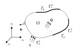
Consider a body occupying an open domain Ω in space that is bounded by a closed surface G as shown in Fig. 1. Material properties are assumed isotropic in domain Ω. The boundaries are composed of a temperature boundary Γ⁰_T, a flux boundary Γ¹_T, a convection boundary Γ²_T, and Γ⁰_T∪ Γ¹_T∪Γ²_T = Γ. Also, the boundaries are mutually disjointed. The body is subjected to the rate of internal heat generation Q and the following thermal boundary conditions. A prescribed temperature T₀ on Γ⁰_T, a prescribed heat flux q on Γ¹_T in the inward normal direction, and an ambient temperature T_∞ on the convection boundary Γ²_T are imposed. is an outward unit vector normal to the boundaries.

https://cdn.apub.kr/journalsite/sites/jcoseik/2015-028-01/02TK022015280102/images/10.7734.28.1.9.F177.png

Figure 1

Body in space

For a temperature field T, a heat conduction equation in steady state is written as

- κT,_{i i} = Q (i = 1, 2, 3)

(1)

where κ is a positive thermal conductivity corresponding to the principal axes and assumed to be independent of temperature. (·),_i represents a partial derivative with respect to the i-coordinate. The notation of repeated subscripts stands for the summation operation over the indices. Three kinds of boundary conditions are applied on the surface of the body as

T = T_{0} on Γ_{T}^{0}

(2)

κT,_{i} n_{i} = q on Γ_{T}^{1}

(3)

κT,_{i} n_{i} + h (T - T_{∞}) = 0  on Γ_{T}^{2}

(4)

where h is a positive convection coefficient on the convection boundary. Space Y for the trial solution is defined as

Y = {\bar{T \in H^{1} (Ω)} : T = T_{0} on Γ_{T}^{0}}

(5)

where H¹ denotes a Hilbert space of order one. Also, space for virtual temperature fields is defined as

\bar{Y} = {\bar{\bar{T} \in H^{1} (Ω)} : \bar{T} = 0 on Γ_{T}^{0}}

(6)

Using the virtual temperature field that satisfies homogeneous boundary conditions, a weak form of Equation (1) is written as

\int_{Ω}^{} (- κ, T_{, i i} - Q) \bar{T} d Q = 0 for  all \bar{T} \in \bar{Y}

(7)

Note that Equation (7) implies the “principle of virtual power” and is independent of time since the steady state problems are considered. Integrating Equation (7) over a unit time leads to the “principle of virtual work” and yields an identical expression. Thus, we regard Equation (7) as a principle of virtual work hereafter. Using the boundary conditions in Equations (2)~(4), Equation (7) can be written as

\int_{Ω}^{} κ, δ_{i j} T_{, i} {\bar{T}}_{, j} d Ω - \int_{Ω}^{} \bar{T} d Ω - \int_{Γ_{T}^{1}}^{} \bar{qT} d Γ

(8)

$+ \int_{Γ_{T}^{2}}^{} h (T - T_{∞}) \bar{T} d Γ = 0$

$f o r all. \bar{T} \in \bar{Y}$

Defining a bilinear thermal energy form

A (T, \bar{T}) = \int_{Ω}^{} T_{, i} κ, δ_{i j} \bar{T_{, j}} d Ω + \int_{Γ_{T}^{2}}^{} h T \bar{T} d Γ

(9)

and a linear load form

L (\bar{T}) = \int_{Ω}^{} Q \bar{T} d Ω + \int_{Γ_{T}^{1}}^{} q \bar{T} d Γ + \int_{Γ_{T}^{2}}^{} h T_{∞} \bar{T} d Γ

(10)

Equation (8) can be written as

Find T∈Y such that

A (T, \bar{T}) = L (\bar{T}) for  all \bar{T} \in \bar{Y}

(11)

3. Continuum-based design sensitivity analysis

3.1 Direct differentiation method

Consider a non-shape design variable vector u that consists of the thermal conductivity of each element. Fora given design u, Equation (11) can be written as

Find T∈Y such that

A_{u} (T, \bar{T}) = L_{u} (\bar{T}) for  all \bar{T} \in \bar{Y}

(12)

where the subscript u indicates the dependence of the abstract form on the design variation. A variational equation corresponding to the perturbed design u+γδu is written as

A_{u + τδu} (T, \bar{T}) = L_{u + τδu} (\bar{T}) for  all \bar{T} \in \bar{Y}

(13)

Using Equation (13), the first order variations of each term in Equation (12) with respect to its explicit dependence on the design variable u are defined as

{A'}_{δu} (T, \bar{T}) = \frac{d}{d τ} L_{u + τδu} (\tilde{T_{τ,}} \bar{T}) |_{τ = 0}

(14)

{L'}_{δu} (\bar{T}) = \frac{d}{d τ} L_{u + τδu} (\bar{T}) |_{τ = 0}

(15)

where the ‘~’ denotes that the dependence on design variation is suppressed. Note that is independent of γ since it is an arbitrary virtual temperature field that belongs to .

Consider the solution of Equation (12). Define the first order variation of the solution with respect to the design u as

T' = \frac{d}{d τ} T (u + τδu) |_{τ = 0} = \lim_{τ \to 0} \frac{T (u + τδu) - T (u)}{τ}

(16)

Using the chain rule of differentiation and the Equation (14), the following holds

\frac{d}{d τ} [A_{u + τδu} (T (u + τδu), \bar{T})] |_{τ = 0}

(17)

$= {A'}_{δu} (T, \bar{T}) + A_{u} (T', \bar{T})$

Using Equations (15) and (17) and taking the first order variation of Equation (12), we have

A_{u} (T', \bar{T}) = {L'}_{δu} (\bar{T}) - {A'}_{δu} (T, \bar{T}) for  all \bar{T} \in \bar{Y}

(18)

Next, consider a general performance functional that may be written, in an integral form, as

Ψ = \int_{Ω}^{} g_{1} (u, T, \nabla T) d Ω + \int_{Ω}^{} g_{2} (u, T, \nabla T) d Γ

(19)

Taking the first order variation of Equation (19), we have the following expression.

Ψ = \frac{d}{d τ}

(20)

$[\begin{matrix} \int_{Ω}^{} g_{1} {u, τδu,T (u + τδu), \nabla T (u + τδu)} d Ω \\ + \begin{matrix} \int_{Ω}^{} g_{2} {u, τδu,T (u + τδu), \nabla T (u + τδu)} d Γ \end{matrix} \end{matrix}]$

$\begin{matrix} {= \int}_{Ω}^{} g_{1, u} δu + \begin{matrix} g_{1, T} \end{matrix} T' + \begin{matrix} \begin{matrix} g_{1, \begin{matrix} \nabla \end{matrix} T} \end{matrix} \begin{matrix} \nabla \end{matrix} T' \end{matrix}) d Ω \end{matrix}$

$\begin{matrix} {+ \int}_{Γ}^{} g_{2, u} δu + \begin{matrix} g_{2, T} \end{matrix} T' + \begin{matrix} \begin{matrix} g_{2, \begin{matrix} \nabla \end{matrix} T} \end{matrix} \begin{matrix} \nabla \end{matrix} T' \end{matrix}) d Γ \end{matrix}$

Once finding T¹ from Equation (18), we trivially obtain the design sensitivity of performance measure from Equation (20).

3.2 Adjoint variable method

To define an adjoint equation for the heat conduction problems, replace the implicit dependence terms T¹ and ∇T¹ in Equation (20) by a virtual temperature and equate the terms involving to the bilinear thermal energy form to yield the adjoint equation as

\begin{matrix} {A_{u} (λ, \bar{λ}) = \int}_{Ω}^{} (g_{1, T} \bar{λ} + g_{1, \nabla T} \nabla \bar{λ}) d Ω \end{matrix}

(21)

$\begin{matrix} {+ \int}_{Γ}^{} (g_{2, T} \bar{λ} + g_{2, \nabla T} \nabla \bar{λ}) d Γ \end{matrix}$

where the adjoint response λ satisfies the homogeneous boundary condition. Since and , Equation (18) can be rewritten as

\begin{matrix} A_{u} (T',λ) = {L'}_{δu} (λ) - \begin{matrix} {A'}_{δu} (T',λ) \forall λ \in \bar{Y} \end{matrix} \end{matrix}

(22)

Noting that and , Equation (21) can be rewritten as

\begin{matrix} A_{u} (λ,T') = \end{matrix} \int_{Ω}^{} (g_{1, T} T' + g_{1, \nabla T} \nabla T') d Ω

(23)

$\begin{matrix} + \end{matrix} \int_{Γ}^{} (g_{2, T} T' + g_{2, \nabla T} \nabla T') d Γ$

$for all T' \in \bar{Y}$

Knowing that A_u(·,·) is a symmetric operator, the following holds.

A_{u} (T', λ) = A_{u} (λ, T')

(24)

Equations (22) and (23) are equivalent and so we can write the following equation.

\int_{Ω}^{} (g_{1, T} T' + g_{1, \nabla T} \nabla T') d Ω

(25)

$+ \int_{Γ}^{} (g_{2, T} T' + g_{2, \nabla T} \nabla T') d Γ = {L'}_{δu} (λ) - {A'}_{δu} (T,λ)$

Substituting Equation (25) into (20), we have

Ψ' = \int_{Ω}^{} g_{1, u} δudΩ + \int_{Γ}^{} g_{2, u} δudΓ + {L'}_{δu} (λ) - {A'}_{δu} (T,λ)

(26)

To evaluate the Equation (26), we need not only the original response T but also adjoint response λ. The efficiency and accuracy of Equation (26) will be demonstrated in section 5.

4. Topology Design Optimization

The objective of the topology optimization method is to find an optimal material distribution that minimizes the thermal energy stored in the system under prescribed thermal loadings. The material distribution can be represented using a normalized bulk material density function that has a continuous variation from zero to one, taking the value of 1.0 for solid material and 0.0 for void. For the topology optimization using the finite element method, the structural domain is discretized into NE finite elements and the bulk material densities are assumed constant in each element. The design variable, bulk material density of each element, is associated with the thermal conductivity using the following expression as

κ_{i} = u_{i}^{p} κ_{0} (i = 0, 1, 2. . ., NE)

(27)

0 < u_{m i n} \leq u_{i} \leq 1

(28)

where κ₀ is the thermal conductivity of original material. A penalty parameter P is used to enforce a concentrated distribution of material. The lower bound of material, ρ_min, is introduced to avoid numerical singularity. A topology design optimization problem is stated as

Minimize

Π = \int_{Ω}^{} QTdΩ + \int_{Γ_{T}^{1}}^{} q TdΓ + \int_{Γ_{T}^{2}}^{} h T_{∞} TdΓ

(29)

Subject to

\int_{Ω}^{} udΩ \leq V_{a l l o w b l e}

(30)

where T¹, q, Q, T_∞, and V_allowable are a temperature field, a prescribed heat flux, a rate of internal heat generation, an ambient temperature, and an allowable volume, respectively.

For the topology optimization, it is very important to make the problem convex to obtain a unique optimal solution regardless of initial design. Otherwise, it may have many local minima and thus the optimal result depends on its initial design. If the Hessian of the unconstrained function that consists of the objective function and constraints is positive definite, the optimization problem is convex. In this topology optimization formulation, only linear constraints with respect to the design variables are considered so that the Hessian of the compliance functional affects the convexity of problem. To check the convexity of performance measure of Equation (29), consider the state equation that is equivalent to the Equation (11) as

r (u, T (u)) = f_{i n t} - f_{e x t} = KT - f_{e x t} = 0

(31)

where u, f_int, f_ext, K, and T are the bulk material density, an internal load, an external load, a system matrix, and a response vector, respectively. Taking the derivative of the state equation with respect to the response T leads to

\frac{\partial r}{\partial T} = K

(32)

and with respect to the design variable yields

\frac{d r}{du} = \frac{\partial r}{\partial u} + \frac{\partial r}{\partial T} \frac{d T}{d u} = \frac{\partial r}{\partial u} + K \frac{d T}{d u} = 0

(33)

Taking the derivative of second equality in Equation (31) with respect to the design variable u yields

\frac{d K}{d u} T = - K \frac{d T}{d u} = \frac{\partial r}{\partial u}

(34)

where Equation (33) is used in the second equality. The thermal compliance functional is rewritten in a discretized form

Π = f_{e x t}^{T} T = \frac{1}{2} T^{T} KT

(35)

Taking the derivative of the compliance functional with respect to the design variable u, we have

\frac{d Π}{d u} = T^{T} K (\frac{d T}{d u}) + \frac{1}{2} T^{T} \frac{d K}{d u} T = - \frac{1}{2} T^{T} (\frac{\partial r}{\partial u})

(36)

where Equation (34) is used in the second equality. Taking the derivative of Equation (36) with respect to the design variable u again yields

\frac{d^{2} Π}{d u^{2}} = - \frac{1}{2} {(\frac{d T}{d u})}^{2} (\frac{\partial r}{\partial u}) - \frac{1}{2} T^{T} \frac{d}{d u} (\frac{\partial r}{\partial u})

(37)

$= - \frac{1}{2} {(\frac{\partial r}{\partial u})}^{T} K^{- 1} (\frac{\partial r}{\partial u}) - \frac{1}{2} T^{T} \frac{d}{d u} (\frac{d K}{d u} T)$

The last term of Equation (37) is expressed using Equation (34) as

\frac{1}{2} T^{T} (\frac{d}{d u}) (\frac{d K}{d u} T) = \frac{1}{2} T^{T} \frac{d^{2} K}{d u^{2}} T + \frac{1}{2} T^{T} \frac{dK}{d u} \frac{d T}{d u}

(38)

$= \frac{1}{2} T^{T} \frac{d^{2} K}{d u^{2}} T - \frac{1}{2} {(\frac{\partial r}{\partial u})}^{T} K^{- 1} (\frac{\partial r}{\partial u})$

Thus, Equation (37) can be expressed in terms of the design variable u as

\frac{d^{2} Π}{d u_{i}^{2}} = {(\frac{\partial r}{\partial u})}^{T} K^{- 1} (\frac{\partial r}{\partial u_{i}})

(39)

$- \frac{1}{2} P (P - 1) δ_{i j} T^{T ~} K (u_{j}^{(P - 2)}) T$

where is the second order derivative of matrix with respect to design variable u. If the penalty parameter P is equal to zero or one, the second term in Equation (39) vanishes so that the problem is convex. Otherwise, it may have many local minima.

Since the topology optimization necessarily uses many design variables, gradient-based optimization methods are generally preferred. Therefore, the sensitivity of the performance measures with respect to the design variables should be determined in a very efficient manner. Among various DSA methods, the continuum-based adjoint variable method is known to be most efficient and accurate and thus widely used in topology optimization problems. To derive the adjoint design sensitivity, consider a thermal compliance functional

Ψ = \int_{Ω}^{} g_{1} (u, T, \nabla T) d Ω + \int_{Γ}^{} g_{2} (u, T, \nabla T) d Γ

(40)

$= L_{u} (T) = Π$

=L_u(T)=Π

Taking the first order variation of Equation (29) with respect to the design variables u leads to

Ψ' = \int_{Ω}^{} (g_{1, u} δ u + g_{1, T} T' + g_{1, \nabla T} \nabla T') d Ω

(41)

$+ \int_{Γ}^{} (g_{2, u} δ u + g_{2, T} T' + g_{2, \nabla T} \nabla T') d Γ$

$= \int_{Ω}^{} QT' d Ω + \int_{Γ_{T}^{1}}^{} qT' d Γ + \int_{Γ_{T}^{2}}^{} h T_{∞} T' d Γ$

Thus

{L'}_{δu} (T) = \int_{Ω}^{} g_{1, u} δu d Ω + \int_{Γ}^{} g_{2, u} δu d Γ = 0

(42)

The adjoint equation is written as

A_{u} (λ, \bar{λ}) = \int_{Ω}^{} (g_{1, T} \bar{λ} + g_{1, \nabla T} \nabla \bar{λ}) d Ω

(43)

$+ \int_{Γ}^{} (g_{2, T} \bar{λ} + g_{2, \nabla T} \nabla \bar{λ}) d Γ$

$= \int_{Ω}^{} Q \bar{λ} d Ω + \int_{Γ_{T}^{1}}^{} q \bar{λ} d Γ + \int_{Γ_{T}^{2}}^{} h T_{∞} \bar{λ} d Γ$

Comparing Equation (43) with Equation (11), the following holds.

λ = T

(44)

The compliance sensitivity using Equation (26) is obtained as

Ψ' = \int_{Ω}^{} g_{1, u} δudΩ + \int_{Γ}^{} g_{2, u} δudΓ + {L'}_{δu} (T) - {A'}_{δu} (T,T)

(45)

Using Equation (42), Equation (45) is reduced to

Ψ' = {- A'}_{δu} (T,T) = - \int_{Ω}^{} T_{, u} κ' δ_{i j} T_{, j} dΩ

(46)

5. Numerical Examples

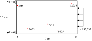
The first example is to verify the DSA method in the temperature field. Consider a rectangular plate (10cm by 5.5cm with thickness of 1.5mm) that consists of 14,080(88 by 160) finite elements with temperature and concentrated heat flux boundary conditions as shown in Fig. 2. Temperature boundary T=0℃ is imposed at 10 elements each on top and bottom of the left side and a heat flux q=133,333(W/m²) is applied at 42 elements on the center of the right side. The thermal conductivity coefficient of aluminum κ=237(W/m·℃) is used in this problem. Design variables are the thermal conductivity coefficients of certain elements as shown in Fig. 2. Performance measure is the thermal compliance of the structure.

Table 1

Comparison of design sensitivity

Design Variable	FDM(a)	AVM(b)	(b)/(a)(%)
κ₃₄₀	-9.3845×10-3	-9.3856×10-3	100.0117
κ₂₆₅₅	-2.5933×10-3	-2.5936×10-3	100.0116
κ₇₂₄₂	-2.0694×10-3	-2.0696×10-3	100.0097
κ₉₄₂₅	-1.9682×10-3	-1.9684×10-3	100.0102
κ₁₂₇₅₃	-8.9883×10-4	-8.9894×10-3	100.0122

https://cdn.apub.kr/journalsite/sites/jcoseik/2015-028-01/02TK022015280102/images/10.7734.28.1.9.F178.png

Figure 2

Rectangular plate

The obtained analytical sensitivity is compared with the finite difference one. In Table 1, the thermal compliance sensitivity with respect to the thermal conductivity of each element is shown. The last column shows the percent agreement between those. Excellent agreements are observed.

Consider the same structure in Fig. 2. This time, the design variables are the thermal conductivity coefficients of all the elements. Performance measure is the thermal compliance of the structure, and allowable volume is 40% of the original one. The final material distribution after the topology optimization is shown in the Fig. 3. As shown in Table 2, the thermal compliance has been decreased to about 70% of the initial one.

https://cdn.apub.kr/journalsite/sites/jcoseik/2015-028-01/02TK022015280102/images/10.7734.28.1.9.F174.png

Figure 3

Topology optimization result

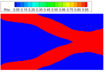
Table 2

Optimization result

	Initial design(a)	Final design(b)	(b)/(a)(%)
Objective function	92.8575	28.1253	30.2887

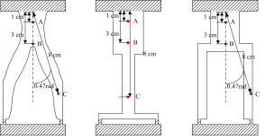
The purpose of topology optimization in heat conduction problems is to find an optimal material layout that yields a thermally stiff structure. To verify the topology optimization results we compare the temperature of the optimal design and two different models generated intuitively , design 1 and design 2, which have an identical volume as shown in Fig. 4. To measure the temperature, a thermal imaging camera VarioCAM head HiRes 640G is used which has 0.03 K thermal resolution. To impose a heat flux boundary condition, q=133,333(W/m²), we utilized a power supply to mainta 50V and 0.22A on a PTC heater. For the temperature boundary condition, T=0℃, we used ice water.

https://cdn.apub.kr/journalsite/sites/jcoseik/2015-028-01/02TK022015280102/images/10.7734.28.1.9.F176.png

Figure 4

Optimal and sample designs

https://cdn.apub.kr/journalsite/sites/jcoseik/2015-028-01/02TK022015280102/images/10.7734.28.1.9.F179.png

Figure 5

Flow chart

https://cdn.apub.kr/journalsite/sites/jcoseik/2015-028-01/02TK022015280102/images/10.7734.28.1.9.F175.png

Figure 6

CAD modeling procedure

https://cdn.apub.kr/journalsite/sites/jcoseik/2015-028-01/02TK022015280102/images/10.7734.28.1.9.F180.png

Figure 7

Manufactured designs

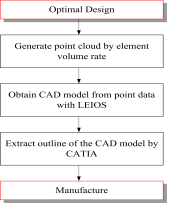
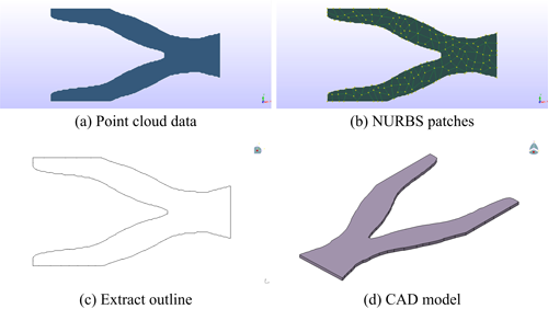
Aluminum is used to manufacture the optimal and two different designs since fabrication is easy and it has sufficient thermal conductivity. The flow chart of manufacturing is shown in Fig. 5. First of all, by using a simple numerical scheme(Lee and Min, 2003), we convert the information of optimal design to point cloud data(Fig. 6(a)). Then we obtain the NURBS(Non Uniform Rational B-Spline) patch model(Fig. 6(b)), by utilizing Leios 2010.1 3D3 Solutions. After that, we transform it into IGES file format with CATIA v5 by Dassault Systems to get the outlines of the model(Fig. 6(c)). Finally we give the thickness to the model for manufacturing(Fig. 6(d)), by using the pad option in CATIA v5. The manufactured optimal and sample designs are shown in Fig. 7.

To experimentally validate the topology design optimization results, we compare the temperature variation of optimal design and two intuitively modeled designs at three different points as shown in Fig. 8. Each point(A, B, C) is located at a certain distance from the flux boundary, 1cm, 3cm, and 8cm, respectively. The temperature contour and variations to time at each point are shown in Fig. 9 and 10. A solid line indicates the temperature variation of optimal design, a dashed line for design 1, and a long dashed line for design 2.

Figure 8

Temperature measuring points

https://cdn.apub.kr/journalsite/sites/jcoseik/2015-028-01/02TK022015280102/images/10.7734.28.1.9.F182.png

https://cdn.apub.kr/journalsite/sites/jcoseik/2015-028-01/02TK022015280102/images/10.7734.28.1.9.F183.png

https://cdn.apub.kr/journalsite/sites/jcoseik/2015-028-01/02TK022015280102/images/10.7734.28.1.9.F184.png

Figure 9

Temperature contours at each point

https://cdn.apub.kr/journalsite/sites/jcoseik/2015-028-01/02TK022015280102/images/10.7734.28.1.9.F185.png

Figure 10

Temperature variations at each point

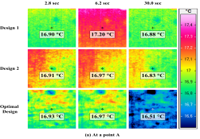
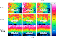
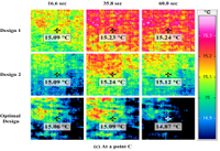
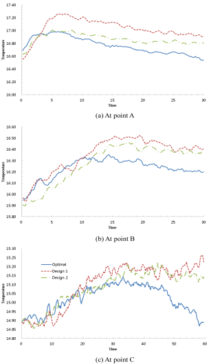
At points A and B, we measured the temperature for 30 seconds when it seemed to reach the steady state. Initially at both points, as the heat propagates, the temperature increases in all three designs. However, the optimal design shows the smallest increase of temperature for points A and B. This means that it is harder to increase the temperature and it decreases the temperature at both points more quickly than the other two designs so that it has the lowest temperature when it seems to reached the steady state. At point C, we measured the temperature for 60 seconds since it is located farther than the other two points. Also, it is located near the temperature boundary T=0℃, so physically it should release temperature more quickly to lower the temperature of the entire system. After 35 seconds, the optimal design decreases the temperature of the point when the other two designs maintains or even increases the temperature at point C. Therefore, based on the experiment, we can verify that the optimal design obtained from topology optimization for minimizing the thermal compliance is the best layout to make it difficult to increase the temperature and to quickly disperse the heat in the system for the given loading and boundary conditions than the other designs.

6. Conclusions

In this study, we have experimentally validated that the optimal design from topology optimization for heat conduction problems has the best material layout to minimize the thermal compliance of the system for given loading and boundary conditions. Experiments have been carried out by utilizing commercial softwares to model a CAD model of the optimal design to manufacture and by using a high resolution thermal imaging camera to measure temperature quantities at certain points. Through the experiment, by comparing the temperature variation of system to time, it turns out that the optimal topology design is harder and faster to increase and release the temperature of system than the other designs modeled intuitively.

Acknowledgements

This research was supported by Basic Science Research Program through the National Research Foundation of Korea(NRF) funded by the Ministry of Education, Science and Technology(Grant Number 2010-18282). The support is gratefully acknowledged. The authors would also like to thank Ms. Inyoung Cho at Korea University for editing assistance.

References

Bendsøe, M.P., Kikuchi, N.1988Generating Optimal Topologies in Structural Design using a Homogenization MethodComput. Methods Appl. Mech. &Eng.711972242810.1016/0045-7825(88)90086-2

Cho, S., Jung, H.2003Design Sensitivity Analysis and Topology Optimization of Displacement-loaded Nonlinear StructuresComput. Methods Appl. Mech. &Eng.192253925532810.1016/S0045-7825(03)00274-3

Haug, E.J., Choi, K.K., Komkov, V.1986Design Sensitivity Analysis of Structural Systems, Academic PressNewYork83109

Kim, M.G., Kim, J.H., Cho, S.2010Topology Design Optimization of Heat Conduction Problems using Adjoint Sensitivity Analysis MethodJ. Comput. Struct. Eng. Inst. Korea236683691

Li, Q., Steven, Querin, S.O.M., Xie, Y.M.1999Shape and Topology Design for Heat Conduction by Evolutionary Structural OptimizationInt. J. Heat &Mass Trans.42336133712810.1016/S0017-9310(99)00008-3

Sluzalec, A., Kleiber, M.1996Shape Sensitivity Analysis for Nonlinear Steady-state Heat Conduction ProblemsInt. J. Numer. Methods Eng.3926092810.1016/0017-9310(95)00237-52613

Tortorelli, D.A., Haber, R.B., Lu, S.C-Y. 1989aDesign Sensitivity Analysis for Nonlinear Thermal SystemsComput. Methods Appl. Mech. &Eng.7761772810.1016/0045-7825(89)90128-X

Journal of the Computational Structural Engineering Institute of Korea ISSN:1229-3059(Print) 2287-2302(Online) 한국전산구조공학회 논문집

Preview

Topology Design Optimization and Experimental Validation of Heat Conduction Problems

ABSTRACT

MAIN

Figure 1

Body in space

Table 1

Comparison of design sensitivity

Figure 2

Rectangular plate

Figure 3

Topology optimization result

Table 2

Optimization result

Figure 4

Optimal and sample designs

Figure 5

Flow chart

Figure 6

CAD modeling procedure

Figure 7

Manufactured designs

Figure 8

Temperature measuring points

Figure 9

Temperature contours at each point

Figure 10

Temperature variations at each point

Acknowledgements

References