

1. Introduction
Atom-based molecular dynamics(MD) simulations are very useful in analyzing nano-scale phenomena which cannot be captured in a continuum sense. However, atomistic simulation tools themselves are not sufficient for many of the interesting and fundamental problems that arise in computational mechanics, since the length and time scales used in the MD simulations are still limited. Many multiscale analysis methods have been developed considering both the MD and the continuum analyses to solve the problems such as dislocation (Tadmor and Ortiz, 1996), crack propagation(Park et al., 2005; Farrell et al., 2007), and strain localization(Kadowaki and Liu, 2007) which cannot be solved with only continuum- based concept. The main issue of multiscale problems is how to connect the atom-level simulations to continuum-level. Bridging scale method(BSM)(Wagner and Liu, 2003) is introduced by deriving dynamic multiscale boundary conditions as a damping force using the generalized Langevin equation(GLE)(Adelman and Doll, 1974, 1976). They used the MD in a localized region of interest and the finite element method in a global region by decoupling the fine and coarse scales through a mass-weighted projection. This boundary condition prevents the wave reflection in the fine scale without any handshake or scale down regions.
Mathematically, design sensitivity analysis(DSA) methods are well developed based on continuum mechanics for structural systems(Choi and Kim, 2004). Since the MD is one of transient dynamic problems, DSA for transient dynamic problems is indispensible for the design of nano- and micro- scale problems. However, a huge amount of compu-tation is usually required for the MD simulations since they are transient dynamic problems. For the DSA of MD systems that have many design varia-bles, the computational cost is very expensive. Therefore, an efficient and accurate analytical DSA method is necessary in the problems that include molecular dynamics analysis. However, the DSA in the multiscale analysis is not straightforward, since the sensitivity relationship between the scales is not well known yet. Even though the relations are known, iterative sensitivity computations might be necessary between the fine and coarse scales depending on the multiscale decomposition method. Therefore, for an efficient DSA in the multiscale problems, it is important to choose the decom-position method that could provide fully decoupled scales in the DSA. In this research, we suggest an analytical DSA method using a BSM to avoid the aforementioned difficulties in the multiscale problems including the MD simulations. The BSM defines the fine scale as the solution whose projection onto the coarse scale basis functions vanishes; this implies the orthogonality between the fine and coarse scales. In addition, the projection operator used in the BSM gives fully decoupled multiscale equations, which enables us to avoid iterative computations between the scales and to perform efficient DSA in the multiscale problems.
2. Review of Bridging Scale Method
The bridging scale method was developed to couple atomistic and continuum scale simulation (Wagner and Liu, 2003). The main idea is to decompose the total displacement  into coarse and fine scales as
 (1)
(1)
The coarse scale displacement is defined as
 (2)
(2)
where  is the shape function of node
  at point
  , and
, and  is the FE nodal displacement corresponding to node
  . In MD simulation, MD displacement
  is regarded as the exact solution. The fine scale displacement is simply that part of the total displacement that the coarse scale cannot represent, and then the error is defined as
 (3)
(3)
which means mass-weighted square of the fine scale, and a temporary nodal solution  is determined to minimize the error, which yields
 (4)
(4)
where  is a diagonal atomic mass matrix, and
  . Then, the fine scale displacement
  is written as
 (5)
(5)
where the projection matrix P is defined as
 (6)
(6)
Finally, the total displacement is rewritten as
 (7)
(7)
where the complimentary projector  .
.
3. Generalized Langevin Equation
A free vibration equation is generally written as
 (8)
(8)
 is a displacement field at time
  ,
,  is a mass matrix, and
  is a stiffness matrices. Then we can solve Eq. (8) using the velocity verlet algorithm,
 (9a)
(9a)
 (9b)
(9b)
 (9c)
(9c)
 (9d)
(9d)
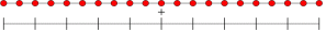
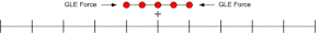
Consider an one-dimensional atomic chain shown in Fig. 1. (a) and (b) show a full MD system and a reduced one, respectively.
For simplicity,  and
and  are given as
 ,
, 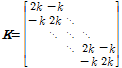 (10)
(10)
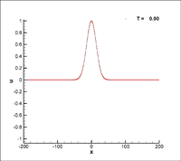
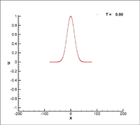
where  1, and the initial condition is given as Gaussian type distribution as


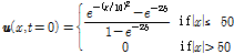 (11)
(11)
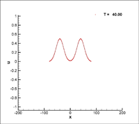
Simulation results for the full MD system are plotted in Fig. 2. It is observed that the initial wave propagates smoothly in both directions.
Assume that displacement  is partitioned into two parts, i.e.
  is the solution of interest, whose degrees of freedom will be kept, and
  is the solution to be mathematically replaced by boundary forces. In this example, the interface between and lies at
  80. Then Eq. (8) is decomposed into those two parts as
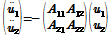 (12)
(12)
where  . If we merely regard as zero, then we have
 (13)
(13)
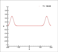
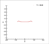
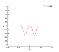
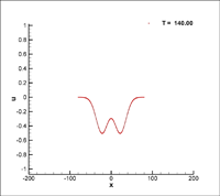
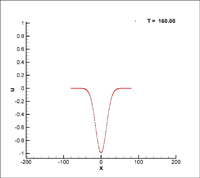
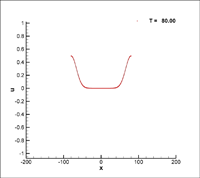
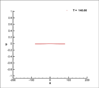
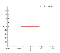
When a reduced system is introduced only between  =±80 without GLE force, this approach causes an unwanted boundary wave reflection as Fig. 3.
At time  160, the same wave as the initial condition is reflecting with reverse phase. Instead, we introduce generalized Langevin equation to remove boundary reflection. First of all, the degrees of freedom are eliminated by solving Eq. (12) and substituting the result back into the equation for .
 (14)
(14)
To obtain  explicitly, the Laplace transform is introduced. The Laplace transform of a function
  , defined for all real numbers
  0, is the function
  defined by
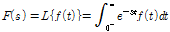 (15)
(15)
where the Laplace operator  transforms time domain
  into space domain
  . The inverse Laplace transform is given by the following complex integral
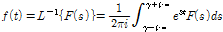 (16)
(16)
where  is a real number so that the contour path of integration is in the region of convergence of
  normally requiring
  for every singularity
  of
of  . Using the definition of the Laplace transformation as Eq. (15), the following properties can be derived:
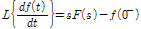 (17a)
(17a)
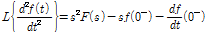 (17b)
(17b)
and another useful property of the Laplace transform is the convolution property as
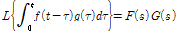 (18)
(18)
Applying Eq. (17b) into Eq. (14) gives
 (19)
(19)
Rearranging Eq. (19) yields
 (20)
(20)
where the matrix  can be written as
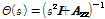 (21)
(21)
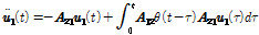
Taking the inverse Laplace transform on Eq. (20) and using the convolution rule, the equation for  is derived as
 (22)
(22)
where the time history kernel  is
is
 (23)
(23)
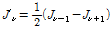
For given mass and stiffness matrices and , is derived analytically(Wagner and Liu, 2003)
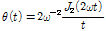 (24)
(24)
where  is a first-kind second-order Bessel function, and
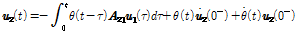
  . Substituting Eq. (22) into Eq. (12) yields the equation for
 (25)
(25)

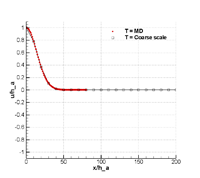
The second to fourth terms in Eq. (25) are the GLE forces and prevent boundary reflections. As shown in Fig. 4, the initial wave passes smoothly through the boundary and no reflection happens.


Then, the generalized Langevin equation(GLE) is utilized to simulate a coupled MD-continuum equation. The bridging scale method is applicable to the problems where the MD region is confined to a small portion of the domain, while the continuum region exists in the whole domain. It may be possible to solve the full MD system, but it requires huge amount of computational cost, especially in 2- or 3-dimensional case. The advantage of bridging scale method is that one can precisely solve the specific region of interest using MD simulation, and bridge MD solution with continuum solution at the MD-continuum boundary. Also, the fine scale waves in MD region pass the boundary smoothly into continuum region by GLE force.
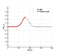
Consider one-dimensional MD-continuum coupled simulation(Park and Liu, 2004) as shown in Fig. 5. The entire domain is -200 200, and the MD particles lie at -8080.
In brief, the coupled MD/FE equations of motion are described as

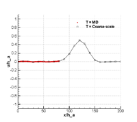
 (26)
(26)
 (27)
(27)
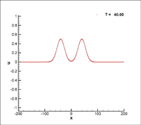
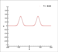
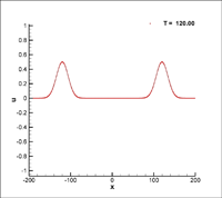
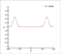
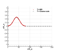
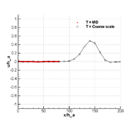
In Fig. 6 and 7, the solid and void dots denote the positions of MD particles and FE nodal points, respectively. From the initial condition, a wave is propagating in both directions. Due to symmetry, the solution at  0 is plotted in all the figures. In Fig. 6, GLE force is applied at MD-continuum boundary and the initial wave passes out of the MD region smoothly without any boundary reflections.


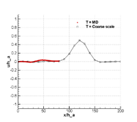
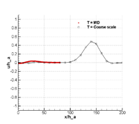
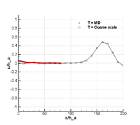
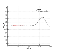
However, if the boundary condition is simply applied by setting the MD velocity at the boundary equal to the coarse scale velocity, the fine scale waves cannot pass through the MD-continuum boundary and undesirable wave reflections occur at the boundary as shown in Fig. 7.
4. Design Sensitivity Analysis
Assume that  has zero initial condition as
 (28)
(28)
Then, Eq. (25) is rewritten as
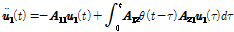 (29)
(29)
4.1 Perturbation of  by 0.1%
The design sensitivity equation for is obtained from the derivative of Eq. (29) with respect to stiffness k as
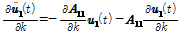 (30)
(30)
Using velocity verlet algorithm, the displacement sensitivity  is updated. The derivative
  is easily obtainable, and is already available from the dynamic solution of Eq. (8). The accuracy of design sensitivity of displacement is verified in Table 1. For each time step , the analytic sensitivity is compared with the finite difference sensitivity. In the last column, very good agreement is observed at every time step.
Table 1
Design sensitivity agreement at x=0
4.2 Perturbation of all  by 0.1%
The design sensitivity equation for is obtained from the derivative of Eq. (29). Unlike Eq. (30), there are more design dependent terms as
 (31)
(31)

Table 2
Design sensitivity agreement at x=0
The derivatives  ,
,  and
and  are easily obtainable, and is already available from the dynamic solution of Eq. (8). Using the relation
 (32)
(32)
the derivative of time history kernel is derived as
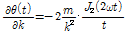 (33)
(33)
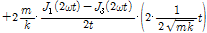
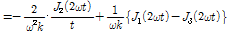
The accuracy of design sensitivity of displacement is also verified in Table 2. For each time step t, the analytic sensitivity is compared to the finite difference sensitivity. In the last column, good agreement is observed at every time step.
5. Conclusions
A multi-scale DSA method is developed using a bridging scale approach. To avoid any iterative computations between the scales, we use a fully decoupled equation for each scale in original response as well as sensitivity analyses. Through a GLE, a locally confined MD region instead of whole MD system is considered for the fine scale solution whereas a FE analysis for the coarse scale solution is performed on the whole region. The efficiency of the developed method is achieved due to the fully decoupled multi- scale equations in these scales, which are derived using identical mass-weighted projection in the response analysis. Numerical implementations demonstrate the accuracy of the developed DSA method for various design variables. The developed method turns out to work very well for any design variable in both scales.
