A Stress-Based Gradient Elasticity in the Smoothed Finite Element Framework

Changkye Lee; Sundararajan Natarajan

doi:10.7734/COSEIK.2024.37.3.187

Preview

Research Paper

Journal of the Computational Structural Engineering Institute of Korea. 30 June 2024. 187-195
https://doi.org/10.7734/COSEIK.2024.37.3.187

A Stress-Based Gradient Elasticity in the Smoothed Finite Element Framework

평활화 유한요소법을 도입한 응력기반 구배 탄성론

Changkye Lee¹^*

Sundararajan Natarajan²

이 창계¹^*

Sundararajan Natarajan²

¹Postdoctoral Research Associate, Division of Cardiovascular Medicine, University of Miami, Florida, 33130, USA

²Professor, Department of Mechanical Engineering, Indian Institute of Technology Madras, Chennai, 600036, India

¹미국 마이애미대학교 의과대학 박사후연구원

²인도 마드라스공과대학 기계공학과 교수

^{*Corresponding Author}

License (open-access, http://creativecommons.org/licenses/by-nc/3.0/):

This is an Open-Access article distributed under the terms of the Creative Commons Attribution Non-Commercial License (http://creativecommons.org/licenses/by-nc/3.0) which permits unrestricted non-commercial use, distribution, and reproduction in any medium, provided the original work is properly cited.

ABSTRACT

This paper presents two-dimensional boundary value problems of the stress-based gradient elasticity within the smoothed finite element method (S-FEM) framework. Gradient elasticity is introduced to address the limitations of classical elasticity, particularly its struggle to capture size-dependent mechanical behavior at the micro/nano scale. The Ru-Aifantis theorem is employed to overcome the challenges of high-order differential equations in gradient elasticity. This theorem effectively splits the original equation into two solvable second-order differential equations, enabling its incorporation into the S-FEM framework. The present method utilizes a staggered scheme to solve the boundary value problems. This approach efficiently separates the calculation of the local displacement field (obtained over each smoothing domain) from the non-local stress field (computed element-wise). A series of numerical tests are conducted to investigate the influence of the internal length scale, a key parameter in gradient elasticity. The results demonstrate the effectiveness of the proposed approach in smoothing stress concentrations typically observed at crack tips and dislocation lines.

Keywords

smoothed finite element method

gradient elasticity

stress concentration

internal length scale

본 논문에서는 평활화 유한요소법(Smoothed finite element method)을 도입한 응력 기반 구배 탄성론(Gradient elasticity)의 2차원 경계치 문제에 대한 연구를 수행하였다. 구배 탄성론은 기존 탄성론에서는 표현할 수 없는 미소규모의 크기 의존적인 기계적 거동을 설명하기 위해 제안되었다. 구배 탄성체론에서 고차 미분 방정식을 두 개의 2차 미분 방정식으로 분할하는 Ru-Aifantis 이론을 사용하기 때문에 평활화 유한요소법에 적용이 가능하게 된다. 본 연구에서 경계치 문제를 해결하기 위해 평활화 유한 요소 프레임워크에 스태거드 방식(Staggered scheme)을 사용하여 국부 변위장과 비국부 응력장을 평활화 영역 및 요소에서 각각 계산하였다. 구배 탄성에서 중요한 변수인 내부 길이 척도의 영향을 측정하기 위해 일련의 수치 예제를 수행하였다. 수치 해석 결과는 제안한 기법이 내부 길이 척도에 따라 균열 선단과 전위 선에 나타나는 응력 집중을 완화할 수 있음을 보여준다.

키워드

평활화 유한요소법

구배 탄성체

응력 집중

내부 길이 척도

MAIN

1. Introduction
2. Theoretical Background of Gradient Elasticity
3. Smoothed finite element method: overview
4. Numerical tests
4.1 Cantilever beam
4.2 Plate with a U-notched hole
4.3 Plate with a crack
5. Conclusions

1. Introduction

Classical continuum mechanics theories are widely used in various engineering applications. Through all-embracing experiments, it has been found that many engineering materials, e.g. metals, composite, concrete, ceramics, polymers, etc., behave differently when they are of different sizes. Such mechanical behaviors by the size effect have been revealed by the micro-structure of the materials (Kolo, 2019). Classical elasticity theory troubles capturing the mechanical behavior of the size effect often observed at a micro-scale level because their assumption is obviously larger than micro-scale. Therefore, this leads to the development of gradient elasticity which possesses the internal length scale (Tenek and Aifantis, 2001; 2002). The internal length scale represents the information on the micro-structure of materials. However, its physical interpretation still remains with no consensus since it depends on material context.

To properly explain it, various studies have been proposed: strain gradient theory (Aifantis, 1992; Ru and Aifantis, 1993), gradient continua (Auffray et al., 2015), modified couple stress theory (Mindlin, 1964; Toupin, 1962) and non-local elasticity theory (Eringen, 1983; Pisano et al., 2009). These methods have one or more additional constants. Hence, one of the simplest theories including one additional constant to explain the size effect of micro-structures is introduced by Aifantis (1992). Although, in his study, stress concentration was quite removed at the tip of the crack and at the lines of dislocations/disclinations, the treatment of high-order derivatives of gradients in the governing equations was still needed. This is because the higher order derivatives are required $C^{1}$ continuous approximation space within the finite element framework. Later, Ru and Aifantis (1993) introduced the theorem to avoid continuity. In their approach, the fourth-order differential equations are parted into two parts of second-order differential equations. A staggered approach successfully handled boundary value problems of gradient elasticity in the framework of the finite element method (FEM) (Askes et al., 2008).

In this study, instead of FEM, we employ the smoothed finite element method (S-FEM) in the staggered approach for gradient elasticity. The smoothed finite element framework were introduced to improve the quality of the finite element solution obtained when using simplex elements, in particular, on triangles, the S-FEM variants such as the node-based S-FEM (NS-FEM) and edge-based S-FEM (ES-FEM) in 2D and NS-FEM and face-based S-FEM (FS-FEM) in 3D have shown to yield more accurate results than the traditional FEM. While cell-based S-FEM (CS-FEM) theoretically is similar to the traditional FEM and so does not relatively improve the solution over the triangular elements. These merits do come at a cost. The bandwidth of the the bilinear form computed using the ES-FEM/NS-FEM/FS-FEM is larger than the traditional FEM, which in turn increases the storage. However, there is a tradeoff between the desired accuracy and computational cost.

Since Liu et al. (2007a) introduced S-FEM, it has shown its toleration to shear/volumetric locking and heavily distorted meshes (Francis et al., 2022; Jiang et al., 2015; Lee et al., 2017). In addition, S-FEM has solved various engineering problems, in particular, discontinuity (Kshirsagar et al., 2021; Lee et al., 2023a; Surendran et al., 2021). Besides such aspects, S-FEM in general shows fast convergence and yields high accuracy than those of FEM in classical linear elasticity (Bordas and Natarajan, 2010; Liu et al., 2007b). Hence, S-FEM is suitable as a possible candidate for gradient elasticity to draw the size effect for micro-structures. Amongst different strain smoothing schemes, cell-based and edge-based strain smoothing methods are considered in this study.

This paper is organized as follows: the fundamental background of the stress-based gradient elasticity in the framework of finite element approximation is briefly introduced in Section 2 and the overview of smoothed finite element method is revisited in Section 3. Systematic numerical studies are conducted to draw the effect of the internal length scales on gradient elasticity in the context of the proposed S-FEM. Lastly, overall remarkable conclusions are discussed in the last section.

2. Theoretical Background of Gradient Elasticity

In this section, the governing equation and the discretized weak form of stress-based gradient elasticity are briefly discussed. Aifantis and his co-workers (Aifantis, 2003; Altan and Aifantis, 1997) suggested the following simple strong form of gradient elasticity:

(1)

σ = ℂ (1 - l_{0}^{2} \nabla^{2}) ϵ

where 𝜎 is the Cauchy stress, the infinitesimal strain is represented by $ϵ = \frac{1}{2} (\nabla u + \nabla u^{T})$ , $ℂ$ is the elastic modulus, $l_{0}$ is a material length parameter/internal length scale which relates to micro-structural characteristics and $u$ is the displacement field. The equilibrium equations for a homogeneous body in the absence of inertia and body force is given by: $\nabla σ = 0$ . Then the fourth-order system of equation is derived as:

(2)

\frac{1}{2} ℂ [\nabla^{2} u + \nabla^{2} u^{T} - l_{0}^{2} \nabla^{2} (\nabla^{2} u + \nabla^{2} u^{T})]

Note that to solve Eq. (2) numerical technique needs $C^{1}$ continuous shape functions. However, by virtue of Ru-Aifiantis theorem, Eq. (2) can be rewritten in such $C^{0}$ continuous shape functions are required. The corresponding weak form is:

(3)

\int_{Ω} ϵ (v)^{T} σ (u) d Ω = \int_{Γ} v^{T} \hat{t} d Γ

where $u$ is the trial function, $v$ is the test function and $\hat{t}$ is the traction. By substituting Eq. (1) to Eq. (3), we can obtain:

(4)

\int_{Ω} ϵ (v)^{T} ℂ (1 - l_{0}^{2} Ω^{2}) ϵ (u) d Ω = \int_{Γ} v^{T} \hat{t} d Γ

Then, we can derive Eq. (4) by applying integration by part on the higher-order term to get the following equation:

(5)

\int_{Ω} ϵ (v)^{T} ℂ ϵ (u) d Ω + \int_{Ω} \nabla ϵ (v)^{T} l_{0}^{2} ℂ \nabla ϵ (u) d Ω = \int_{Γ} v^{T} \hat{t} d Γ + \int_{Γ} ϵ (v)^{T} l_{0}^{2} ℂ ϵ (u) d Ω

Note that in a $C^{1}$ continuous formulation, it is typical to assume that this higher-order boundary condition vanishes at the boundary (Askes and Aifantis, 2002). However, in this study, due to the use of operator split, the higher-order boundary condition also vanishes as a result of the chosen boundary conditions. Then, Eq. (5) leads to $K u = f$ (the system of linear equations), where:

(6a)

K = \sum_{e} K^{e} = \sum_{e} [\int_{Ω^{h}} B^{T} ℂ B d Ω + \int_{Ω^{h}} \nabla B^{T} l_{0}^{2} ℂ \nabla B d Ω]

(6b)

f = \sum_{e} f^{e} = \sum_{e} \int_{Γ_{t}} v^{T} \hat{t} d Γ

where $B$ is the strain-displacement matrix. In the current approach, the strain-displacement matrix $B$ is built over smoothing domains, while traditionally it is computed on elements. The detailed computation of the $B$ matrix will be discussed in Section 3.

To solve Eq. (6), Ru and Aifantis (1993) introduced the operator split approach. In the context of finite element implementation, this approach includes two steps: computation of local displacements and computation of non-local stress fields. Firstly, the computation of local displacement fields is the same as classical elasticity as follows:

(7)

K u = [\int_{Ω} B^{T} ℂ B d Ω] u = f

Once, the local displacement field is obtained, the non-local stress is calculated as:

(8)

σ^{g} - l_{0}^{2} \nabla^{2} σ^{g} = ℂ L u

where the non-local stress $σ^{g}$ is a nodal unknown field and $L$ is the linear differential operator given as in 2D:

(9)

L = [\begin{array}{cc} \frac{\partial}{\partial x} & 0 \\ 0 & \frac{\partial}{\partial y} \\ \frac{\partial}{\partial y} & \frac{\partial}{\partial x} \end{array}]

The weak form of Eq. (8) can be given by:

(10)

\int_{Ω} (v^{T} σ^{g} + \nabla v^{T} l_{0}^{2} \nabla σ^{g}) d Ω = \int_{Ω} v^{T} ℂ L u d Ω

where $σ^{g} = \sum N_{I} s_{I}^{g}$ with a set of shape functions $N$ as given in Eq. (11) and the nodal non-local stress $s_{I}^{g}$ .

(11)

N = [\begin{array}{ccc} N_{I} & 0 & 0 \\ 0 & N_{I} & 0 \\ 0 & 0 & N_{I} \end{array}], I = 1, \dots, n

where $n$ is the number of nodes of the element. Finally, Eq. (10) can be rewritten using Eq. (1) and the non-local stress definition as follows:

(12)

[\int_{Ω} (N^{T} N + l_{0}^{2} \frac{\partial N^{T}}{\partial \hat{x}} \frac{\partial N}{\partial \hat{x}}) d Ω] s^{g} = \int_{Ω} N^{T} ℂ L u d Ω

where a summation $\hat{x} = x, y$ . In this paper, we utilise the smoothed finite element method, which will be discussed in Section 3, to solve the local displacement field and use the finite element method to get the non-local stress. Interested readers can refer to Bagni and Askes (2015) and Lee et al. (2023b) and references therein for further details.

3. Smoothed finite element method: overview

In this section, the basic idea behind the gradient smoothing approach in the framework of the finite element method is briefly revisited. Liu et al. (2007a) introduced the gradient smoothing approach in the framework of the finite element method, often called smoothed finite element method (S-FEM) to improve linear triangular and bilinear quadrilateral elements. The one of remarkable aspects of S-FEM is the sub-division of finite elements, so-called sub-cells. Then, sub-cells are reconstructed to smoothing domains by different schemes where gradients are smoothed over the smoothing domains. Hence, strains are continuous over the smoothing domains but are discontinuous across the boundaries of smoothing domains, not elements (Liu and Nguyen, 2016).

Fig. 1 illustrates two main schemes of S-FEM that how to construct the smoothing domains: cell-based and edge-based S-FEM. Fig. 1(a) explains the concept of cell-based S-FEM (CS-FEM) and Fig. 1(b) is about edge-based S-FEM (ES-FEM), respectively. As shown in Fig. 1, each 3-node triangular element is split into three triangular sub-cells. Then, in the cell-based scheme, for example, $∆ 234$ is divided into three sub-cells: $∆ 23 O_{2}$ , $∆ 34 O_{2}$ and $∆ 24 O_{2}$ . In CS-FEM, each sub-cell becomes the smoothing domain where strains will be smoothed. ES-FEM also needs to split triangular elements into three triangular sub-cells. However, the smoothing domain is built by the position of the target edge. For instance, as shown in Fig. 1(b), when the target edge $k$ that the sharing boundary of $∆ 123$ and $∆ 234$ is chosen, the smoothing domain is combined by a sub-cell $∆ 23 O_{1}$ of $∆ 123$ and a sub-cell $∆ 23 O_{2}$ of $∆ 234$ . Note that, when the target edge is the boundary of the domain, only one sub-cell is used as the smoothing domain in ES-FEM since the edge does not have a neighboring finite element.

https://cdn.apub.kr/journalsite/sites/jcoseik/2024-037-03/N0040370305/images/Figure_jcoseik_37_03_05_F1.jpg

Fig. 1.

Construction of smoothing domains for each cell-based and edge-based scheme

In S-FEM approximation, the following infinitesimal strain ${\tilde{ϵ}}^{h}$ over the smoothing domain $Ω_{k}$ is considered:

(13)

{\tilde{ϵ}}^{h} (x_{k}) = \int_{Ω_{k}} ϵ^{h} (x) Φ (x) d Ω, \forall x \in Ω_{k}

where a point $x_{k}$ is located on the boundaries of the smoothing domain and the weight function 𝛷 is given in Eqs. (14a) and (14b):

(14a)

\int_{Ω_{k}} Φ (x) d Ω = 1, Φ > 0

(14b)

Φ (x) = \{\begin{cases} \begin{array}{ll} 1 / A_{k} & x \in Ω_{k} \end{array} \\ \begin{array}{ll} 0 & x \notin Ω_{k} \end{array} \end{cases}

Hence, Eq. (13) can be rewritten by means of the divergence theorem as follows:

(15)

ϵ (x_{k}) = \frac{1}{A_{k}} \int_{Ω_{k}} ϵ (x) Φ (x) d Ω = \frac{1}{A_{k}} \int_{Γ_{k}} n (x) u^{h} (x) d Ω

where $A_{k}$ is the area of the smoothing domain and $n (x)$ is the outward normal vector given at Gauss points located on the middle point of boundaries of the smoothing domain as shown in Fig. 1. In terms of the nodal displacements, Eq. (15) is rewritten as:

(16)

\tilde{ϵ} (x) = \sum_{I \in G_{k}} \tilde{B_{I}} (x) u_{I}^{h}

where $G_{k}$ is a set of nodes. The 2D smoothed strain-displacement matrix from Eq. (16) is defined as follows:

(17)

{\tilde{B}}_{I R} = [\begin{array}{cc} {\tilde{B}}_{I x} & 0 \\ 0 & {\tilde{B}}_{I y} \\ {\tilde{B}}_{I y} & {\tilde{B}}_{I x} \end{array}]

where

(18)

{\tilde{B}}_{I i} = \frac{1}{A_{k}} \int_{Γ_{k}} N_{I} (x) n_{i} (x) d Γ

(19)

n = [\begin{array}{cc} n_{x} & 0 \\ 0 & n_{y} \\ n_{y} & n_{x} \end{array}]

where $N_{I}$ is the shape functions and $Γ_{k}$ is the boundaries of the smoothing domain and Eq. (19) denotes the 2D matrix form of the outward normal vectors. Since the 2D matrix form of the outward normal vectors is equivalent to the differential operator (Eq. (9)), Eq. (17) can be utilized for the computation of the stiffness matrix in the same manner as in FEM. As shown in Fig. 1 and Eq. (18), the proposed S-FEM does not require an explicit form of shape functions. In other words, there is no isoparametric mapping. In addition, the interior Gauss integration is altered to line integration with one Gauss point at the middle of boundaries of the smoothing domain (please refer to Fig. 1). These salient features of S-FEM bring marked benefits that it can avoid over-estimation of the stiffness and is immune to highly distorted meshes.

The discrete system equations for S-FEM is given by:

(20)

\begin{aligned} \tilde{K} u = f \\ \tilde{K} = \int_{Ω} {\tilde{B}}^{T} (x) \tilde{ℂ B} (x) d Ω = \sum_{k = 1}^{n} \int_{Ω_{k}} {\tilde{B}}^{T} (x) ℂ B (x) d Ω \\ = \sum_{k = 1}^{n} {\tilde{B}}^{T} (x) \tilde{ℂ B} (x) A_{k} \end{aligned}

where $n$ is the number of target cells/edges for each scheme. The external force vector $f$ is obtained in the same manner in finite element approximation. In the present approximation, Eq. (7) is replaced by Eq. (20) for the local displacement fields. Eq. (12) is applied to each finite element in the current framework to obtain the non-local stress field.

4. Numerical tests

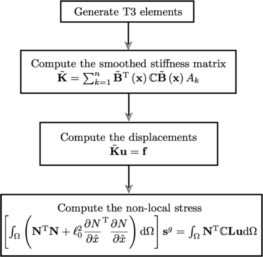
This section presents a series of two-dimensional tests with the proposed CS-FEM and ES-FEM. Fig. 2 illustrates the main process of the present framework. After generating triangular finite meshes, the smoothed stiffness matrix is constructed on either cell-based smoothing domains or edge-based smoothing domains. The non-local stress field is then calculated element-wise using Eq. (12).

https://cdn.apub.kr/journalsite/sites/jcoseik/2024-037-03/N0040370305/images/Figure_jcoseik_37_03_05_F2.jpg

Fig. 2.

Schematic steps for the computation of displacements and non-local stress

A cantilever beam subject to end shear is validated to show the accuracy of the proposed S-FEM, compared to the analytical solution. Then, to capture the size effect at the dislocation lines and crack tip, a plate with a U-notched hole under far-field tension and a plate with a crack are examined. For all examples, 3-node triangular finite element meshes are used. To discuss the results, we use the following conventions:

∙ CS-FEM: cell-based smoothed finite element method

∙ ES-FEM: edge-based smoothed finite element method

∙ T3: 3-node triangular element

∙ DOFs: degrees of freedom

To examine tests, the proposed framework has been coded in MATLAB 2023b and the implementation was conducted on an Apple M2 chip with a clock speed of 3.49 GHz and 16 GB of memory.

4.1 Cantilever beam

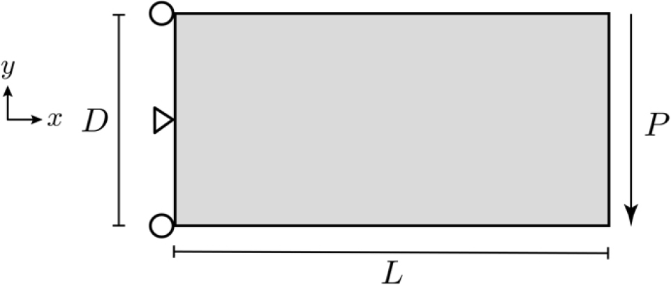
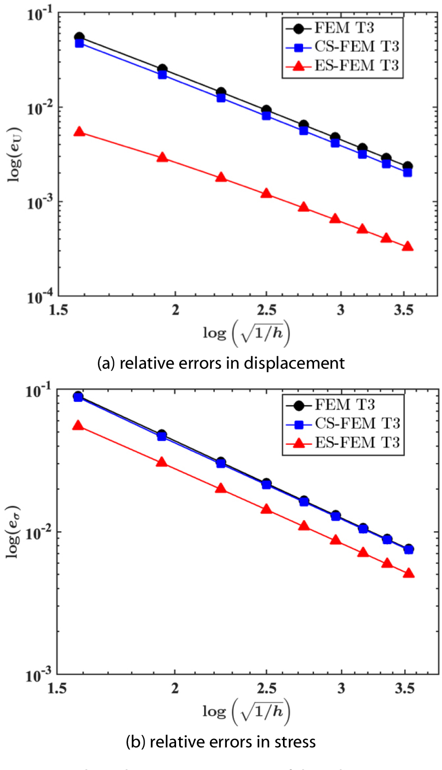
This section tests a cantilever beam as the validation for the proposed smoothed FEM. Fig. 3 depicts the geometry of the beam and boundary conditions. The length of the beam is $L \in 0, 5$ m and the height is given as $D \in - 1, 1$ m. The boundary conditions are imposed on the left end of the beam and the load $P$ =1 N carries on the right side of the beam. Young’s modulus and Poisson’s ratio are $E$ =1000 N/m² and 𝜐=0.3, respectively. Note that the internal length scale is $l_{0}$ =0.0. The exact displacements and stresses can be found in Augarde and Deeks (2008): $σ_{x x} = \frac{P (L - x) y}{I}, σ_{y y} = 0, τ_{x y} = - \frac{P}{2 I} (\frac{D^{2}}{4} - y^{2}), u_{x} = - \frac{P y}{6 E I} [(6 L - 3 x) x + (2 + υ) (y^{2} - \frac{D^{2}}{4})]$ and $u_{y} = - \frac{P}{6 E I} [3 υ y^{2} (L - x) + (4 + 5 υ) \frac{D^{2} x}{4} + (3 L - x) x^{2}]$ . For this test, the following 9 levels of refined T3 elements are used: 306, 650, 1122, 1722, 2450, 3306, 4290, 5402 and 6642 DOFs. Fig. 4 shows the convergence of displacements and stresses for FEM, CS-FEM and ES-FEM. As expected, CS-FEM provides marginally better results in displacements and stresses to FEM; while ES-FEM yields more accurate results than other approaches.

https://cdn.apub.kr/journalsite/sites/jcoseik/2024-037-03/N0040370305/images/Figure_jcoseik_37_03_05_F3.jpg

Fig. 3.

Geometry and boundary conditions of a cantilever beam

https://cdn.apub.kr/journalsite/sites/jcoseik/2024-037-03/N0040370305/images/Figure_jcoseik_37_03_05_F4.jpg

Fig. 4.

Cantilever beam: convergence of the relative errors in displacements and stresses for FEM and S-FEM

4.2 Plate with a U-notched hole

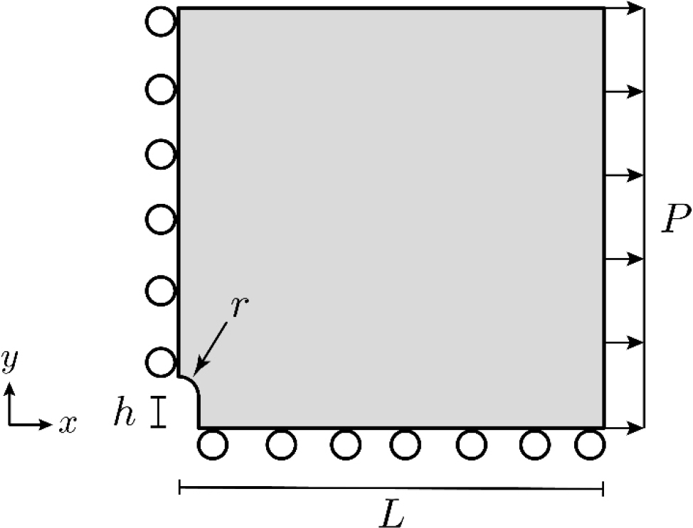
Next, the infinite plate with a U-notched hole with the lateral extension is considered. As shown in Fig. 5, the length and height of the plate are $L$ =5 m with the height of notch $h$ =0.1 m and the radius of the hole is $r$ =0.1 m, respectively. Lateral tension $σ_{x x} = 10^{3}$ N/m² is implemented on the right edge of the plate. The same material properties used in Section 4.1 are also used for this test.

https://cdn.apub.kr/journalsite/sites/jcoseik/2024-037-03/N0040370305/images/Figure_jcoseik_37_03_05_F5.jpg

Fig. 5.

Geometry and boundary conditions of an infinite plate with U-notched hole

It is known that the infinite plate with a hole shows the stress concentration at the top of the hole because of a geometric discontinuity. Hence to quantify the effect of the stress concentration by the internal length scale, we measure the stress concentration factor $K_{t}$ given as (Pilkey and Pilkey, 2008):

$K_{t} = \frac{σ_{m a x}}{σ_{n o m}} = C_{1 +} C_{2} (\frac{h}{t}) + C_{3} (\frac{h}{t})^{2 +} C_{4} (\frac{h}{t})^{3}$

where for $0.1 \leq h / r \leq 2.0$ , $C_{1} = 0.955 + 2.169 \sqrt{h / r} - 0.081 h / r, C_{2} = - 1.557 - 4.046 \sqrt{h / r} + 1.032 h / r, C_{3} = 4.013 + 0.424 \sqrt{h / r} - 0.748 h / r$ and $C_{4} = - 2.461 + 1.538 \sqrt{h / r} - 0.236 h / r$ . $σ_{m a x}$ is obtained at the top of the notch where $y = h + r$ . Therefore, the stress concentration factor of the plate is $K_{t}$ =3.656.

Fig. 6 shows the convergence of the stress concentration factors with respect to the length of the plate and the internal length scales, $l_{0}$ ={0.001,0.005,0.01,0.05,0.1,0.5,1.0}. As shown in Fig. 6, ES-FEM gives a more accurate $K_{t}$ than CS-FEM. Furthermore, $K_{t}$ of both methods is decreased when the internal length scales are close to 1.0.

https://cdn.apub.kr/journalsite/sites/jcoseik/2024-037-03/N0040370305/images/Figure_jcoseik_37_03_05_F6.jpg

Fig. 6.

Convergence of the stress concentration factor $K_{t}$ with respect to the internal length scale $l_{0}$

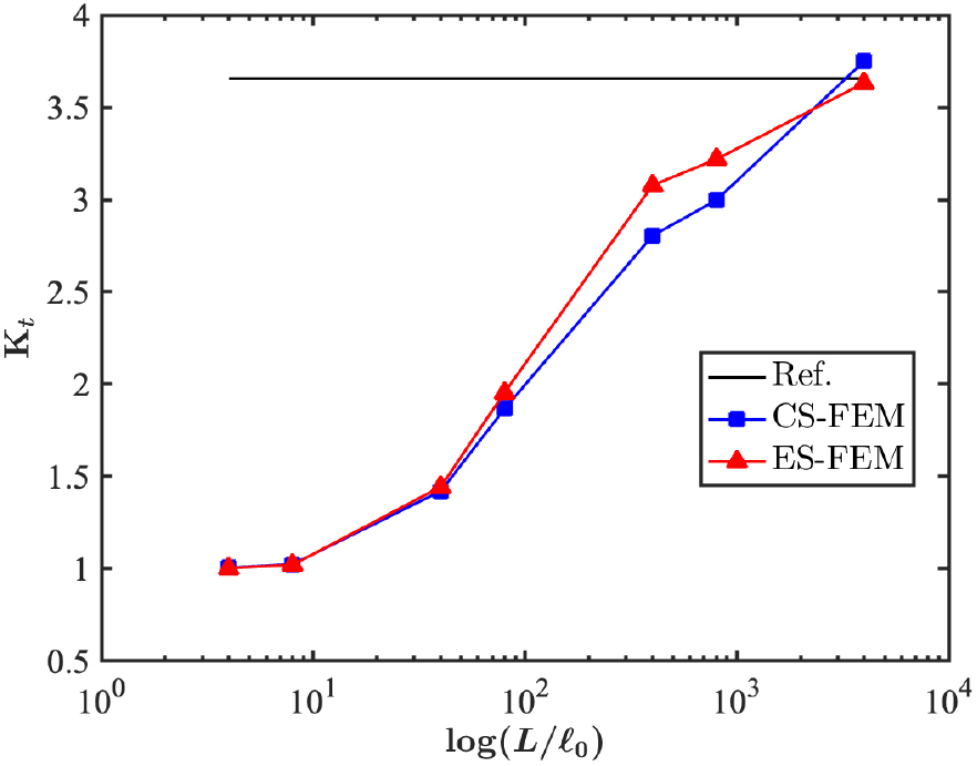
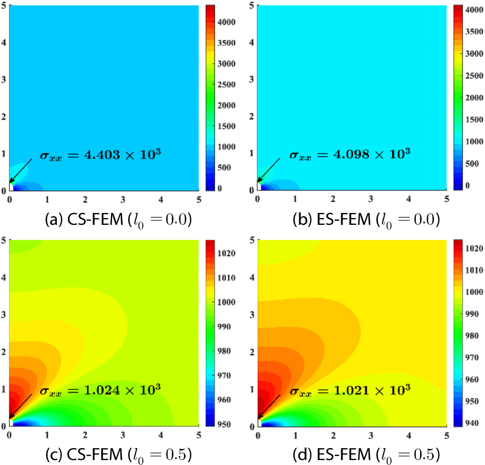
Fig. 7 illustrates stress $σ_{x x}$ distribution with the different length scales, $l_{0}$ =0.0 and $l_{0}$ =0.5. Figs. 7(a) and 7(b) show the stress distribution when $l_{0}$ =0.0, i.e. the classical elasticity. Figs. 7(c) and 7(d) show the distribution of stress for CS-FEM and ES-FEM when $l_{0}$ =0.5. It can be found that when the internal length scale is increased, the stress concentration is vanished and the values of stress are dramatically decreased.

https://cdn.apub.kr/journalsite/sites/jcoseik/2024-037-03/N0040370305/images/Figure_jcoseik_37_03_05_F7.jpg

Fig. 7.

Stress $σ_{x x}$ distribution for a plate with a U-notched hole for $l_{0}$ =0.0 and $l_{0}$ =0.5

4.3 Plate with a crack

Lastly, to verify the relaxation of stress concentration in stress-based gradient elasticity, we consider a plate with a crack, as shown in Fig. 8. The plate is a rectangular shape with dimensions of $L$ =1 mm and the bottom edge is fully constrained. The crack implies as $d$ =0.3 mm at $y$ =1.0 mm. Two different material properties are assigned to two regions: (a) the left half ( $x$ =0~0.5 mm) has Young’s modulus $E_{1}$ =17 GPa and Poisson’s ratio $v_{1}$ =0.15 and (b) the right half ( $x$ =0.5~1.0 mm) has Young’s modulus $E_{2}$ =200 GPa and Poisson’s ratio $v_{2}$ =0.3, respectively. For this study, 8 different levels of the internal length scales are evaluated: $l_{0}$ ={0.0,0.001,0.005,0.01,0.05,0.1,0.5,1.0}. Both CS-FEM and ES-FEM simulations use 25600 elements (26130 DOFs).

https://cdn.apub.kr/journalsite/sites/jcoseik/2024-037-03/N0040370305/images/Figure_jcoseik_37_03_05_F8.jpg

Fig. 8.

Geometry and boundary conditions of a plate with a crack

Fig. 9 presents the stress distributions obtained using CS-FEM and ES-FEM for different internal length scales (51,842 degrees of freedom). As expected, the stress is highly concentrated at the crack tip and the bi-material interface. However, with increasing internal length scale, the stress becomes more evenly distributed throughout the domain, demonstrating the smoothing effect of the internal length scale in the proposed gradient elasticity.

https://cdn.apub.kr/journalsite/sites/jcoseik/2024-037-03/N0040370305/images/Figure_jcoseik_37_03_05_F9.jpg

Fig. 9.

Stress $σ_{y y}$ distribution at the crack tip and the interface of materials for $l_{0}$ =0.001 and $l_{0}$ =0.1

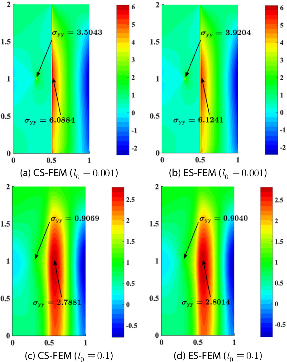
Fig. 10 depicts the stress concentration reduction along the midlines of the plate ( $y$ =1.0 mm) for CS-FEM and ES-FEM. As expected, high stress concentrations are initially observed at the crack tip and the material interface, as shown in Fig. 10. However, the effect of the internal length scale becomes evident as the stress concentration alleviates. Notably, when the internal length scale approaches $l_{0}$ =0.5, the stress distribution becomes finite, indicating a complete absence of sharp stress gradient.

https://cdn.apub.kr/journalsite/sites/jcoseik/2024-037-03/N0040370305/images/Figure_jcoseik_37_03_05_F10.jpg

Fig. 10.

Stress $σ_{y y}$ at the midline ( $y$ =1.0 mm) of the plate with different internal scale lengths $l_{0}$ =0.0~0.5

5. Conclusions

This paper introduces CS-FEM and ES-FEM for two-dimensional stress-based gradient elasticity. The effectiveness of the proposed framework is demonstrated through various standard problems, consistently yielding accurate results. The influence of the internal length scale on stress concentration is investigated. The versatility of the framework is showcased by its applicability to problems with both smoothed and singular solutions. In particular, a single crack problem with bi-material properties is analyzed. Here, the internal length scale effectively mitigates the singularity typically observed at the crack tip and material interface. The proposed methods offer several advantages:

∙ avoids the need for explicit shape functions, thus, simplifying implementation;

∙ staggered scheme suits local displacement and non-local stress field computations, enhancing computational efficiency;

∙ implementation requires any further human intervention into the existing FEM code for gradient elasticity framework.

However, the proposed approach generally yields a higher computational cost than the standard FEM when employing the same number of DOFs. This increased cost derives from the subdivision of each finite element into sub-domains, which are utilized to construct smoothing domains. Consequently, the proposed S-FEM exhibits a wider stiffness bandwidth than FEM.

In future work, the application of gradient elasticity to functionally graded materials within the context of stress-constrained structural topology optimization will be explored.

References

Aifantis, E.C. (1992) On the Role of Gradients in the Localization of Deformation and Fracture, Int. J. Eng. Sci., 30, pp.1279~1299.

10.1016/0020-7225(92)90141-3

Aifantis, E.C. (2003) Update on a Class of Gradient Theories, Mech. Mater., 35, pp.259~280.

10.1016/S0167-6636(02)00278-8

Altan, B.S., Aifantis, E.C. (1997) On Some Aspects in the Special Theory of Gradient Elasticity, J. Mech. Behav. Mater., 8, pp.231~282.

10.1515/JMBM.1997.8.3.231

Askes, H., Aifantis, E.C. (2002) Numerical Modeling of Size Effects with Gradient Elasticity - Formulation, Meshless Discretization with Examples, Int. J. Fract., 117, pp.347~358.

10.1023/A:1022225526483

Askes, H., Morata, I., Aifantis, E.C. (2008) Finite Element Analysis with Staggered Gradient Elasticity, Comput. & Struct., 86, pp.1266~1279.

10.1016/j.compstruc.2007.11.002

Auffray, N., dell'Isola, F., Eremeyev, V.A., Madeo, A., Rosi, G. (2015) Analytical Continuum Mechanics à la Hamilton-Piola: Least Action Principle for Second Gradient Continua and Capillary Fluids, Math. & Mech. Solids, 20, pp.375~417.

10.1177/1081286513497616

Augarde, C.E., Deeks, A.J. (2008) The Use of Timoshenko's Exact Solution for a Cantilever Beam in Adaptive Analysis, Finite Elem. Anal. & Des., 44, pp.595~601.

10.1016/j.finel.2008.01.010

Bagni, C., Askes, H. (2015) Unified Finite Element Methodology for Gradient Elasticity, Comput. & Struct., 160, pp.100~110.

10.1016/j.compstruc.2015.08.008

Bordas, S.P.A., Natarajan, S. (2010) On the Approximation in the Smoothed Finite Element Method (SFEM), Int. J. Numer. Methods Eng., 81, pp.660~670.

10.1002/nme.2713

Eringen, A.C. (1983) On Differential Equations of Nonlocal Easticity and Solutions of Screw Dislocation and Surface Waves, J. Appl. Phys., 54, pp.4703~4710.

10.1063/1.332803

Francis, A., Natarajan, S., Lee, C.K., Budarapu, P.R. (2022) A Cell-based Smoothed Finite Element Method for Finite Elasticity, Int. J. Comput. Methods Eng. Sci. & Mech., 23, pp.536~550.

10.1080/15502287.2022.2030427

Jiang, C., Liu, G.R., Han, X, Zhang, Z.-Q., Zeng, W. (2015) A Smoothed Finite Element Method for Analysis of Anisotropic Large Deformation of Passive Rabbit Ventricles in Diastole, International Journal for Numerical Methods in Biomedical Engineering, 31, pp.e02697.

10.1002/cnm.269725382158

Kolo, I. (2019) Computational Gradient Elasticity and Gradient Plasticity with Adaptive Splines, PhD Thesis, University of Sheffield.

Kshirsagar, S., Lee, C.K., Natarajan, S. (2021) -Finite Element Method for Frictionless and Frictional Contact Including Large Deformation, Int. J. Comput. Methods, 18, pp.215002.

10.1142/S021987622150002X

Lee, C.K., Angela Mihai, L., Hale, J.S., Kerfriden, P., Bordas, S.P.A. (2017) Strain Smoothing for Compressible and Nearly-Incompressible Finite Elasticity, Comput. & Struct., 182, pp.540~555.

10.1016/j.compstruc.2016.05.004

Lee, C.K., Natarajan, S., Yee, J.-J. (2023a) Quasi-brittle and Brittle Fracture Simulation Using Phase-field Method based on Cell-based Smoothed Finite Element Method, J. Comput. Struct. Eng. Inst. Korea, 36, pp.295~305.

10.7734/COSEIK.2023.36.5.295

Lee, C.K., Singh, I.V., Natarajan, S. (2023b) A Cell-based Smoothed Finite-Element Method for Gradient Elasticity, Eng. Comput., 39, pp.925~942.

10.1007/s00366-022-01734-2

Liu, G.R., Dai, K.Y., Nguyen, T.T. (2007a) A Smoothed Finite Element Method for Mechanics Problems, Comput. Mech., 39, pp.859~877.

10.1007/s00466-006-0075-4

Liu, G.R., Nguyen, T.T. (2016) Smoothed Finite Element Methods, CRC Press, Boca Raton.

10.1201/EBK1439820278

Liu, G.R., Nguyen, T.T., Dai, K.Y., Lam, K.Y. (2007b) Theoretical Aspects of the Smoothed Finite Element Method (SFEM), Int. J. Numer. Methods Eng., 71, pp.902~930.

10.1002/nme.1968

Mindlin, R.D. (1964) Micro-Structure in Linear Elasticity, Archive for Rational Mechanics and Analysis, 16, pp.51~78.

10.1007/BF00248490

Pilkey, W.D., Pilkey, D.F. (2008) Peterson's Stress Concentration Factors, Wiley, New York.

10.1002/9780470211106

Pisano, A.A., Sofi, A., Fuschi, P. (2009) Nonlocal Integral Elasticity: 2D Finite Element Based Solution, Int. J. Solids & Struct., 46, pp.3836~3849.

10.1016/j.ijsolstr.2009.07.009

Ru, C.Q., Aifantis, E.C. (1993) A Simple Approach to Solve Boundary-Value Problem in Gradient Elasticity, Acta Mech., 101, pp.59~68.

10.1007/BF01175597

Surendran, M., Lee, C.K., Nguyen-Xuan, H., Liu, G.R., Natarajan, S. (2021) Cell-based Smoothed Finite Element Method for Modelling Interfacial Cracks with Non-Matching Grids, Eng. Fract. Mech., 242, p.107476.

10.1016/j.engfracmech.2020.107476

Tenek, L.T., Aifantis, E.C. (2001) On Some Applications of Gradient Elasticity to Composite Materials, Compos. Struct., 53, pp.189~197.

10.1016/S0263-8223(01)00003-4

Tenek, L.T., Aifantis, E.C. (2002) A Two-dimensional Finite Element Implementation of a Special Form of Gradient Elasticity, Comput. Model. Eng. & Sci., 3, pp.731~741.

Toupin, R.A. (1962) Elastic Materials with Couple-Stresses, Arch. Ration. Mech. & Anal., 11, pp.385~414.

10.1007/BF00253945

Journal of the Computational Structural Engineering Institute of Korea ISSN:1229-3059(Print) 2287-2302(Online) 한국전산구조공학회 논문집

Preview

A Stress-Based Gradient Elasticity in the Smoothed Finite Element Framework

ABSTRACT

MAIN

(1)

(2)

(3)

(4)

(5)

(6a)

(6b)

(7)

(8)

(9)

(10)

(11)

(12)

Fig. 1.

Construction of smoothing domains for each cell-based and edge-based scheme

(13)

(14a)

(14b)

(15)

(16)

(17)

(18)

(19)

(20)

Fig. 2.

Schematic steps for the computation of displacements and non-local stress

Fig. 3.

Geometry and boundary conditions of a cantilever beam

Fig. 4.

Cantilever beam: convergence of the relative errors in displacements and stresses for FEM and S-FEM

Fig. 5.

Geometry and boundary conditions of an infinite plate with U-notched hole

Fig. 6.

Convergence of the stress concentration factor Kt with respect to the internal length scale l0

Fig. 7.

Stress σxx distribution for a plate with a U-notched hole for l0=0.0 and l0=0.5

Fig. 8.

Geometry and boundary conditions of a plate with a crack

Fig. 9.

Stress σyy distribution at the crack tip and the interface of materials for l0=0.001 and l0=0.1

Fig. 10.

Stress σyy at the midline (y=1.0 mm) of the plate with different internal scale lengths l0=0.0~0.5

References

Convergence of the stress concentration factor $K_{t}$ with respect to the internal length scale $l_{0}$

Stress $σ_{x x}$ distribution for a plate with a U-notched hole for $l_{0}$ =0.0 and $l_{0}$ =0.5

Stress $σ_{y y}$ distribution at the crack tip and the interface of materials for $l_{0}$ =0.001 and $l_{0}$ =0.1

Stress $σ_{y y}$ at the midline ( $y$ =1.0 mm) of the plate with different internal scale lengths $l_{0}$ =0.0~0.5